
An evolutionary information from SNE to t-SNE and UMAP

Introduction
In accordance with a number of estimates, 80% of information generated by companies immediately is unstructured knowledge similar to textual content, photographs, or audio. This knowledge has huge potential for machine studying purposes, however there’s some work to be completed earlier than it may be used immediately. Function extraction helps extract data from the uncooked knowledge into embeddings. Embeddings, which I coated in a earlier piece with my co-author and Arize colleague Aparna Dhinakaran, are the spine of many deep studying fashions; they’re utilized in GPT-3, DALL·E 2, language fashions, speech recognition, advice programs, and different areas. Nonetheless, one persistent downside is that it’s arduous to troubleshoot embeddings and unstructured knowledge immediately. It’s difficult to grasp this sort of knowledge, not to mention acknowledge new patterns or modifications. To assist, there are a number of distinguished methods to visualise the embedding illustration of the dataset utilizing dimensional discount strategies. On this piece, we’ll undergo three in style dimensionality discount strategies and their evolution.
It’s price noting on the outset that the tutorial papers introducing these strategies — SNE (“Stochastic Neighbor Embedding” by Geoffrey Hinton and Sam Roeweis), t-SNE (“Visualizing Information utilizing t-SNE” by Laurens van der Maaten and Geoffrey Hinton), and UMAP (“Umap: Uniform manifold approximation and projection for dimension discount” by Leland McInnes, John Healey, and James Melville) — are price studying in full. That mentioned, these are dense papers. This piece is meant to be a digestible information — possibly a primary step earlier than studying the whole papers — for time-strapped ML practitioners to assist them perceive the underlying logic and evolution from SNE to t-SNE to UMAP.

What Is Dimensionality Discount?
Dimension discount performs an essential function in knowledge science as a basic method in each visualization and pre-processing for machine studying. Dimension discount strategies map excessive dimensional knowledge X={x0, x1, …, xN} into decrease dimensional knowledge Y = {y0, y1, …, yN} with N being the variety of knowledge factors.
In essence, computing embeddings is a type of dimension discount. When working with unstructured knowledge, the enter house can comprise photographs of measurement WHC (Width, Top, Channels), tokenized language, audio alerts, and so on. As an illustration, let the enter house be composed of photographs with decision 1024×1024. On this case, the enter dimensionality is bigger than a million. Let’s assume you utilize a mannequin similar to ReNet or EfficientNet and extract embeddings with 1000 dimensions. On this case your output house dimensionality is 1000, three orders of magnitude decrease! This transformation turns the very massive, usually sparse, enter vectors into smaller (nonetheless of appreciable measurement), dense function vectors, or embeddings. Therefore, we are going to seek advice from this subspace because the function house or embedding house.
As soon as we’ve function vectors related to our inputs, what can we do with them? How can we get hold of human interpretable data from them? We will’t visualize objects in larger than three dimensions. Therefore, we want instruments to additional scale back the dimensionality of the embedding house down to 2 or three, ideally preserving as a lot of the related structural data of our dataset as potential.
There are an in depth quantity of dimensionality discount strategies. They are often grouped into three classes: function choice, matrix factorization, and neighbor graphs. We’ll concentrate on the latter class, which incorporates SNE (Stochastic Neighbor Embedding), t-SNE (t-distributed Stochastic Neighbor Embedding) and UMAP (Uniform Manifold Approximation and Projection).
Evolution: SNE → t-SNE → UMAP
On this part, we are going to comply with the evolution of neighbor graphs approaches beginning with SNE. Then, we are going to construct from it and clarify the modifications utilized that resulted in t-SNE and afterward in UMAP.
The three algorithms function roughly in the identical manner:
- Compute excessive dimensional chances p.
- Compute low dimensional chances q.
- Calculate the distinction between the chances by a given price operate C(p,q).
- Decrease the price operate.
This part covers the Stochastic Neighbor Embedding (SNE) algorithm. This would be the constructing block from which we’ll develop a greater understanding of t-SNE and UMAP.
Step 1: Calculate the Excessive Dimensional Possibilities
We begin by computing the chance

that the information level i would choose one other level j as its neighbor,
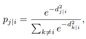
the place

represents the dissimilarity between excessive dimensional factors Xi, Xj. It’s outlined because the scaled Euclidean distance,

Mathematical instinct: Given two factors Xi, Xj, the farther they’re, the upper their distance dj|i, the upper their dissimilarity, and the decrease the chance that they’ll contemplate one another neighbors.
Key idea: the additional away two embeddings are within the house, the extra dissimilar they’re.
Word that the dissimilarities should not symmetric as a result of parameter σi. What’s the that means of this? In apply, the person units the efficient variety of native neighbors or perplexity. As soon as the perplexity, ok, is chosen; the algorithm finds σi by a binary search to make the entropy of the distribution over neighbors equal


the place H is the Shannon entropy, measured in bits. From the earlier equation we are able to get hold of

in order that by tuning σi, we tune the proper hand facet till it matches the perplexity set by the person. The upper the efficient variety of native neighbors (perplexity), the upper σi and the broader the Gaussian operate used within the dissimilarities.
Mathematical instinct: The upper the perplexity, the extra possible it’s to think about factors which can be far-off as neighbors.
One query might come up: if the perplexity is user-determined, how do we all know which one is appropriate? That is the place artwork meets science. The selection of perplexity is essential for a helpful projection right into a low-dimensional house that we are able to visualize utilizing a scatter plot. If we choose too low of a perplexity, clusters of information factors that we count on to be collectively given their similarity won’t seem collectively and we are going to see subclusters as a substitute. Then again, if we choose a perplexity too massive for our dataset, we won’t see appropriate clustering, since factors from different clusters can be thought of neighbors. There isn’t a particular all-good worth for the perplexity. Nonetheless, there are good guidelines of thumb.
Recommendation: The authors of SNE and t-SNE (sure, t-SNE has perplexity as nicely) use perplexity values between 5 and 50.
Since in lots of circumstances there isn’t any technique to know what the right perplexity is, getting probably the most from SNE (and t-SNE) might imply analyzing a number of plots with totally different perplexities.
Step 2: Calculate the Low Dimensional Possibilities
Now that we’ve the excessive dimensional chances, we transfer on to calculate the low dimensional ones, which depend upon the place the information factors are mapped within the low dimensional house. Happily, these are simpler to compute since SNE additionally makes use of Gaussian neighborhoods however with mounted variance (no perplexity parameter),

Step 3: Selection of Value Perform
If the factors Yi are positioned accurately within the low-dimensional house, the conditional chances p and q can be very comparable. To measure the mismatch between each chances, SNE makes use of the Kullback-Leibler divergence as a loss operate for every level. Every level in each excessive and low dimensional house has a conditional chance to name one other level its neighbor. Therefore, we’ve as many loss features as we’ve knowledge factors. We outline the price operate because the sum of the KL divergences over all knowledge factors,

The algorithm begins by inserting all of the yi in random areas very near the origin, after which is educated minimizing the price operate C utilizing gradient descent. Particulars concerning the differentiation of the price operate is past the scope of this publish.
It’s price creating some instinct concerning the loss operate used. The algorithm’s creators state that “whereas SNE emphasizes native distances, its price operate cleanly enforces each protecting the photographs of close by objects close by and protecting the photographs of extensively separated objects comparatively far aside.” Let’s see if that is true utilizing the following determine the place we see the KL divergence for the excessive and low dimensional chances p and q, respectively.

If two factors are shut collectively in excessive dimensional house, their dissimilarities are low and the chance p ought to be excessive (p ~ 1). Then, in the event that they had been mapped far-off, the low dimensional chance can be low (q ~0). On this state of affairs we are able to see that the loss operate takes very excessive values, severely penalizing that mistake. Then again, if two factors are removed from one another in excessive dimensional house, their dissimilarities are excessive and the chance p ought to be low (p0). Then, in the event that they had been mapped close to one another, the low dimensional chance can be excessive (q1). We will see that the KL divergence isn’t penalizing this error as a lot as we’d need. This can be a key problem that can be solved by UMAP.
At this level we’ve a good suggestion of how SNE works. Nonetheless, the algorithm has two issues that t-SNE tries to unravel: its price operate may be very troublesome to optimize, and it has a crowding downside (extra on this beneath). Two primary modifications are launched by t-SNE to unravel these points: symmetrization and using t-distributions for the low-dimensional chances, respectively. These modifications arguably made t-SNE the state-of-the-art for dimension discount for visualization for a few years till UMAP got here alongside.
Symmetric SNE
The primary modification is using a symmetrized model of SNE. Usually, the conditional chances described to this point should not symmetric. Which means the chance of level xi to think about level xj as its neighbor isn’t the identical chance that time xj would contemplate level xi as a neighbor. We symmetrize pairwise chances in excessive dimensional house by defining

This definition of

is such that each knowledge level

makes a non negligible contribution to the price operate. You may be questioning, what concerning the low dimensional chances?
The Crowding Drawback
With what we’ve to this point, if we wish to accurately undertaking shut distances between factors, the reasonable distances are distorted and seem as enormous distances within the low dimensional house. In accordance with the authors of t-SNE, it is because “the world of the two-dimensional map that’s accessible to accommodate reasonably distant knowledge factors won’t be almost massive sufficient in contrast with the world accessible to accommodate close by knowledge factors.”
To resolve this, the second primary modification launched is using the Scholar t-Distribution (which is what provides the ‘t’ to t-SNE) with one diploma of freedom for the low-dimensional chances,

Now the pairwise chances are symmetric

The principle benefit is that the gradient of the symmetric price operate,

has an easier kind and is far simpler and sooner to compute, enhancing efficiency.
Since t-SNE additionally makes use of KL divergence as its loss operate, it additionally carries the issues mentioned within the earlier part. This isn’t to say that it’s utterly ignored, however the principle takeaway is that t-SNE severely prioritizes the conservation of the native construction.
Instinct: For the reason that KL divergence operate doesn’t penalize the misplacement in low dimensional house of factors which can be far-off in excessive dimensional house, we are able to conclude that the worldwide construction isn’t nicely preserved. t-SNE will group comparable knowledge factors collectively into clusters, however distances between clusters won’t imply something.
Uniform Manifold Approximation and Projection (UMAP) for dimension discount has many similarities with t-SNE in addition to some very essential variations which have made UMAP our most popular selection for dimension discount.
The paper introducing the method isn’t for the faint of coronary heart. It particulars the theoretical foundations for UMAP, based mostly in manifold idea and topological knowledge evaluation. We won’t go into the main points of the speculation however preserve this in thoughts: the algorithmic choices in UMAP are justified by sturdy mathematical idea, which in the end will make it such a top quality common objective dimension discount method for machine studying.
Now that we’ve an understanding of how t-SNE works, we are able to construct on that and discuss concerning the variations with UMAP and the results of these variations.
A Graph of Similarities
In contrast to t-SNE that works with chances, UMAP works immediately with similarities.
- Excessive dimensional similarities:

- Low dimensional similarities:

Word that in each circumstances there isn’t any normalization (no denominator) utilized, in contrast to t-SNE, with the corresponding enchancment in efficiency. The symmetrization of the excessive dimensional similarities is carried out utilizing probabilistic t-conorm:

As well as, UMAP permits for various selection of metric features d for the excessive dimensional similarities (eq). We have to deal with the that means of

The previous represents the minimal desired separation between shut factors within the low dimensional house, and the latter is about to be the worth such that

the place ok is the variety of nearest neighbors. Each the
are hyper-parameters with results that can be mentioned on the finish of the part.
Optimization Enhancements
Within the optimization part of the algorithm, the creators of UMAP made some design choices that performed a vital function in its nice efficiency, together with:
- UMAP makes use of cross entropy as loss operate, whereas t-SNE makes use of KL divergence. The CE loss operate has each engaging and repulsive forces, whereas KL solely has engaging (it’s price noting that t-SNE has repulsive forces however not on the loss operate. The repulsive forces seem within the renormalization means of the similarity matrix. Nonetheless, world renormalization may be very costly, UMAP has it less complicated by utilizing CE loss and with higher outcomes on preserving world construction). With this new selection of loss operate, inserting objects which can be far-off in high-dimensional house close by within the low-dimensional house is penalized. Due to the higher selection of loss operate, UMAP can seize extra of the worldwide construction than its predecessors.

Determine: loss operate utilized by t-SNE and UMAP in contrast. The cross-entropy loss (b) penalizes when far-off factors, in excessive dimensional house, are mapped closed collectively within the low dimensional house. The Kullback–Leibler loss (a) fails to do that.
2. UMAP makes use of stochastic gradient descent to reduce the price operate, as a substitute of the slower gradient descent.
Selection of Initialization
UMAP makes use of spectral initialization, not random initialization of the low dimensional factors. A really handy Laplacian Eigenmaps initialization (adopted from the theoretical foundations). This initialization is comparatively fast, since it’s obtained from linear algebra operations. It supplies an excellent start line for stochastic gradient descent. This initialization is, in idea, deterministic. Nonetheless, given the massive sparse matrices concerned, computational strategies present approximate outcomes. As a consequence, determinism isn’t assured however nice stability is achieved. This initialization supplies sooner convergence in addition to larger consistency, i.e., totally different runs of UMAP will yield comparable outcomes.
There are different variations which can be price exploring. Furthermore, UMAP comes with a number of disadvantages. Keep tuned for an upcoming piece on the professionals and cons of UMAP.
Conclusion
Methods for visualizing embeddings have come a good distance up to now few many years, with new algorithms made potential by the profitable mixture of arithmetic, laptop science and machine studying. The evolution from SNE to t-SNE and UMAP opens up new potentialities for knowledge scientists and machine studying engineers to raised perceive their knowledge and troubleshoot fashions.
Wish to be taught extra? Examine monitoring unstructured knowledge and see why getting began with embeddings is simpler than you assume. Any questions? Be happy to achieve out on the Arize group.
