Discover ways to plot your Polars DataFrames
In my earlier article, I talked in regards to the new DataFrame library that’s manner quicker than Pandas — Polars:
A really pure query that comes after that is: what about visualization? Does Polars have visualization capabilities built-in? And so on this article, I’ll present you how one can carry out visualization utilizing Polars DataFrame.
However earlier than I’m going any additional, let me inform you the dangerous information first — Polars doesn’t have plotting capabilities built-in.
At the very least not within the present model (0.13.51). Hopefully in future releases it can combine standard plotting libraries into it.
That stated, you must explicitly plot your Polars DataFrames utilizing a plotting library, reminiscent of matplotlib, Seaborn, or Plotly Specific. For this text, I wish to give attention to utilizing Polars with Plotly Specific for our visualization duties.
The Plotly Python library is an interactive, open supply plotting library. It helps totally different chart sorts masking a variety of statistical, monetary, geographic, scientific, and three-dimensional use-cases. Plotly Specific, alternatively, is a wrapper for the Plotly library, making it simpler so that you can create great-looking charts with out writing an excessive amount of code. The connection between Plotly and Plotly Specific is just like that of matplotlib and Seaborn:

Putting in Plotly Specific
To put in plotly, you possibly can both use pip:
pip set up plotly
Or conda:
conda set up plotly
Let’s create our pattern Polars DataFrame from a dictionary:
import polars as pldf = pl.DataFrame(
{
'Mannequin': ['iPhone X','iPhone XS','iPhone 12',
'iPhone 13','Samsung S11','Samsung S12',
'Mi A1','Mi A2'],
'Gross sales': [80,170,130,205,400,30,14,8],
'Firm': ['Apple','Apple','Apple','Apple',
'Samsung','Samsung','Xiao Mi','Xiao Mi'],
}
)
df

Plotting utilizing matplotlib
For a begin, it could be helpful to plot a bar chart displaying the gross sales of every mannequin. Most information analyst/scientist are aware of matplotlib, and so let’s attempt to use it first:
plt.bar(df['Model'], df['Sales'])
You must see the next output:

The above works as a result of df[‘Model’] and df[‘Sales’] every returns a Polar Sequence, which is appropriate by the bar() methodology of matplotlib. Nonetheless, since sq. bracket indexing is an anti-pattern in Polars, you need to as an alternative use the choose() methodology to pick the columns that you simply wish to plot:
import matplotlib.pyplot as pltplt.bar(
df.choose('Mannequin').to_series(),
df.choose('Gross sales').to_series()
)
Word that you must explicitly convert the results of the
choose()methodology to a Sequence utilizing theto_series()methodology. It is because thechoose()methodology returns a DataFrame.
Plotting utilizing Plotly Specific
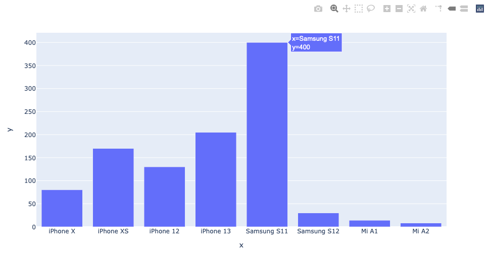
Let’s now plot the bar chart utilizing Plotly Specific:
import plotly.specific as pxpx.bar(x = df.choose('Mannequin').to_series(),
y = df.choose('Gross sales').to_series())
Identical to utilizing matplotlib, it’s essential explicitly move within the columns as a Sequence to the Plotly Specific’s methodology, on this case the bar() methodology.
Plotly Specific shows the bar chart interactively — you possibly can hover over the bars and a popup will show particulars of the bar, and you may as well use the assorted objects within the toolbar to zoom into the chart, save the chart as PNG, and extra:
An alternative choice to plotting the chart utilizing a Polars dataframe is to transform it to a Pandas DataFrame, after which use the Pandas DataFrame immediately with Plotly Specific:
px.bar(df.to_pandas(),     # convert from Polars to Pandas DataFrame
x = 'Mannequin',
y = 'Gross sales')
I’ll use this strategy at any time when it’s extra handy.
If you happen to get an error with the above assertion, it’s essential set up the pyarrow library:
pip set up pyarrow
Plotting a Pie Chart
To plot a pie chart in Plotly Specific, use the pie() methodology:
px.pie(df,                                   # Polars DataFrame
names = df.choose('Mannequin').to_series(),
values = df.choose('Gross sales').to_series(),
hover_name = df.choose('Mannequin').to_series(),
color_discrete_sequence= px.colours.sequential.Plasma_r)
Or in case you are utilizing a Pandas DataFrame:
px.pie(df.to_pandas(),                      # Pandas DataFrame
names = 'Mannequin',
values = 'Gross sales',
hover_name = 'Mannequin',
color_discrete_sequence= px.colours.sequential.Plasma_r)
In both case you will note the next pie chart:

Plotting Line Charts
For this instance, I will probably be utilizing the AAPL-10.csv file from: https://www.kaggle.com/datasets/meetnagadia/apple-stock-price-from-19802021
License — Open Knowledge Commons Open Database License (ODbL) v1.0. Description — This can be a Dataset for Inventory Prediction on Apple Inc. This dataset begin from 1980 to 2021 . It was collected from Yahoo Finance.
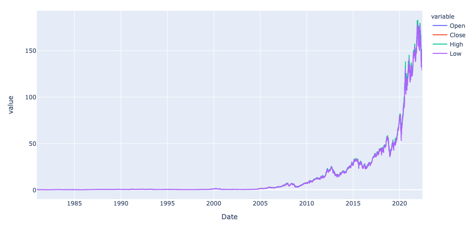
To plot a line chart displaying the Open, Shut, Excessive, and Low costs, it could be simpler to transform the Polars DataFrame on to a Pandas DataFrame and use it within the line() methodology of Plotly Specific:
df = (
pl.scan_csv('AAPL-10.csv')
).gather()px.line(df.to_pandas(),               # covert to Pandas DataFrame
x = 'Date',
y = ['Open','Close','High','Low']
)
The output seems to be like this:
Within the subsequent instance, let’s do some EDA on the Insurance coverage dataset. For this instance, we will use the dataset situated at https://www.kaggle.com/datasets/teertha/ushealthinsurancedataset?useful resource=obtain.
License: CC0: Public Area. Description — This dataset accommodates 1338 rows of insured information, the place the Insurance coverage expenses are given in opposition to the next attributes of the insured: Age, Intercourse, BMI, Variety of Youngsters, Smoker and Area. The attributes are a mixture of numeric and categorical variables.
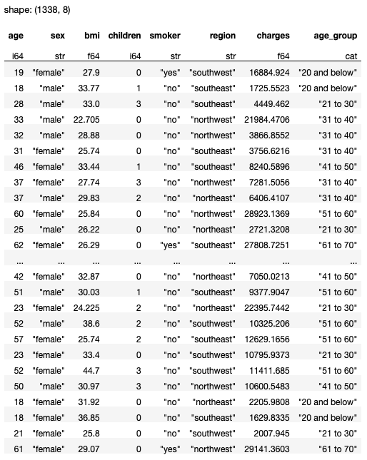
First, load the CSV file as a Polars DataFrame:
import polars as plq = (
pl.scan_csv('insurance coverage.csv')
)df = q.gather()
df

Analyzing the distribution of people who smoke among the many genders
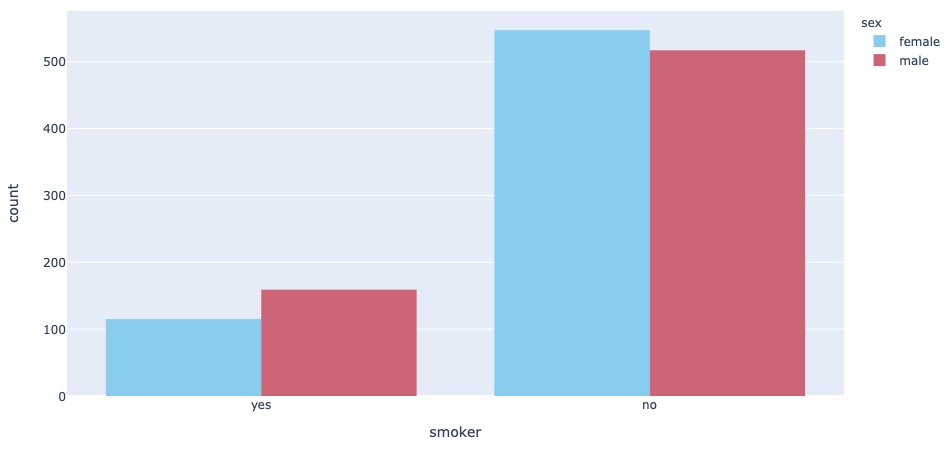
Let’s analyze the distribution of people who smoke for every gender:
import plotly.specific as pxpx.histogram(df.to_pandas(),
x = 'intercourse',
coloration = 'smoker',
barmode = 'group',
color_discrete_sequence = px.colours.qualitative.D3)
As traditional, I discover it simpler to covert the Polars DataFrame to a Pandas Dataframe earlier than I do my plotting. For the plotting, I exploit the histogram() methodology in Plotly Specific. Right here is the output of the above assertion:

As you possibly can see, for every gender, there are extra non-smokers than people who smoke.
Analyzing the distribution of genders among the many people who smoke
Subsequent, we have an interest to see if there are extra male people who smoke or feminine people who smoke:
px.histogram(df.to_pandas(),
x = 'smoker',
coloration = 'intercourse',
barmode = 'group',
color_discrete_sequence = px.colours.qualitative.Protected)
The end result under exhibits that there are extra male people who smoke than feminine people who smoke:
Analyzing how expenses will depend on age
The ultimate evaluation that I wish to do for this dataset is how the costs will depend on age. Because the age column is a steady variable, it could be helpful to have the ability to bin the values into distinct teams after which convert it right into a categorical area. In Polars, you are able to do it utilizing the apply() and solid() strategies:
def age_group(x):
if x>0 and x<=20:
return '20 and under'
if x>20 and x<=30:
return '21 to 30'
if x>30 and x<=40:
return '31 to 40'
if x>40 and x<=50:
return '41 to 50'
if x>50 and x<=60:
return '51 to 60'
if x>60 and x<=70:
return '61 to 70'
return '71 and above'df = df.choose(
[
pl.col('*'),
pl.col('age').apply(age_group).cast(pl.Categorical)
.alias('age_group')
]
)
df
In Pandas, you need to use the
pd.reduce()methodology to performing binning. Sadly there isn’t any equal methodology accessible in Polars.
You’ll get the next output:
Now you can group the dataframe primarily based on the age_group area after which calculate the imply expenses for all of the women and men:
df = df.groupby('age_group').agg(
[
(pl.col('charges')
.filter(pl.col('sex')== 'male'))
.mean()
.alias('male_mean_charges'),
(pl.col('charges')
.filter(pl.col('sex')== 'female'))
.mean()
.alias('female_mean_charges'),
]
).type(by='age_group')
df
You will note the next output:

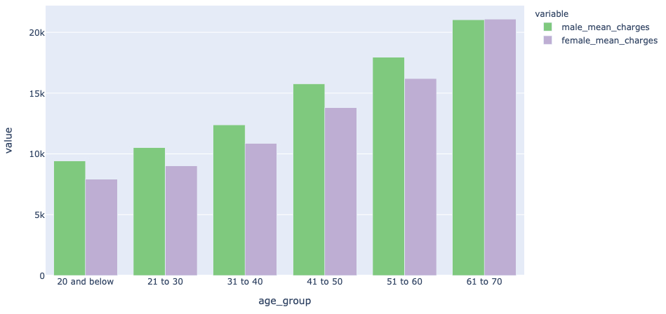
Lastly, now you can plot the chart to indicate how the imply expenses varies for every age group:
px.bar(
df.to_pandas(),
x = "age_group",
y = ['male_mean_charges','female_mean_charges'],
barmode = 'group',
color_discrete_sequence=px.colours.colorbrewer.Accent,
)
Since we’re utilizing Polars, let’s make use of lazy analysis and mix all of the code snippets above right into a single question:
import polars as pldef age_group(x):
if x>0 and x<=20:
return '20 and under'
if x>20 and x<=30:
return '21 to 30'
if x>30 and x<=40:
return '31 to 40'
if x>40 and x<=50:
return '41 to 50'
if x>50 and x<=60:
return '51 to 60'
if x>60 and x<=70:
return '61 to 70'
return '71 and above'q = (
pl.scan_csv('insurance coverage.csv')
.choose(
[
pl.col('*'),
pl.col('age').apply(age_group).cast(pl.Categorical)
.alias('age_group')
]
)
.groupby('age_group').agg(
[
(pl.col('charges')
.filter(pl.col('sex')== 'male'))
.mean()
.alias('male_mean_charges'),
(pl.col('charges')
.filter(pl.col('sex')== 'female'))
.mean()
.alias('female_mean_charges'),
]
).type(by='age_group')
)px.bar(
q.gather().to_pandas(),
x = "age_group",
y = ['male_mean_charges','female_mean_charges'],
barmode = 'group',
color_discrete_sequence=px.colours.colorbrewer.Accent,
)
On this article, you realized that Polars doesn’t include its personal visualization APIs. As an alternative, you must reply by yourself plotting libraries reminiscent of matplotlib and Plotly Specific. When you can immediately move your Polars DataFrame as Sequence to the assorted plotting libraries, it’s generally simpler when you merely convert your Polars DataFrame right into a Pandas DataFrame as most plotting libraries have inherent assist for Pandas.
Sooner or later, it is extremely potential that Polars would have its personal plotting APIs, however for now, you must make do with what you’ve.
