Deep dive within the modelling assumptions and their implications
Whereas digging within the particulars of classical classification strategies, I discovered sparse details about the similarities and variations of Gaussian Naive Bayes (GNB), Linear Discriminant Evaluation (LDA) and Quadratic Discriminant Evaluation (QDA). This publish centralises the knowledge I discovered for the subsequent learner.
Abstract: All three strategies are a particular occasion of The Bayes Classifier, all of them take care of steady Gaussian predictors, they differ within the assumptions they makes concerning the relationships amongst predictors, and throughout lessons (i.e. the best way they specify the covariance matrices).
The Bayes Classifier
Now we have a set X of p predictors, and a discrete response variable Y (the category) taking values okay = {1, …, Okay}, for a pattern of n observations.
We encounter a brand new statement for which we all know the values of the predictors X, however not the category Y, so we want to make a guess about Y based mostly on the knowledge we now have (our pattern).
The Bayes classifier assigns the check statement to the category with the best conditional likelihood, given by:

The place: pi_k is the prior estimate, f_k (x) is our chance. To acquire chances for sophistication okay, we have to outline formulae for the prior and the chance.
The prior. The likelihood of observing class okay, i.e. that our check statement belongs to class okay, with out having additional info on the predictors. Taking a look at our pattern, we are able to consider the circumstances in school okay as realisations from a random variable with Binomial distribution:

the place for n trials, in every trial the statement both belongs (success) or doesn’t belong (failure) to class okay. It may be proven that the relative frequency of successes — the quantity successes over the full variety of trials — is an unbiased estimator for pi_k. Therefore, we use the relative frequency as our prior for the likelihood that an statement belongs to class okay.
The chance: The chances are the likelihood of seeing these values for X, on condition that the statement truly belongs to class okay. Therefore, we have to discover the distribution of the predictors X in school okay. We don’t know what the “true” distribution is, so we are able to’t “discover” it, we relatively make some affordable assumptions about the way it may seem like, after which use our pattern to estimate its parameters.
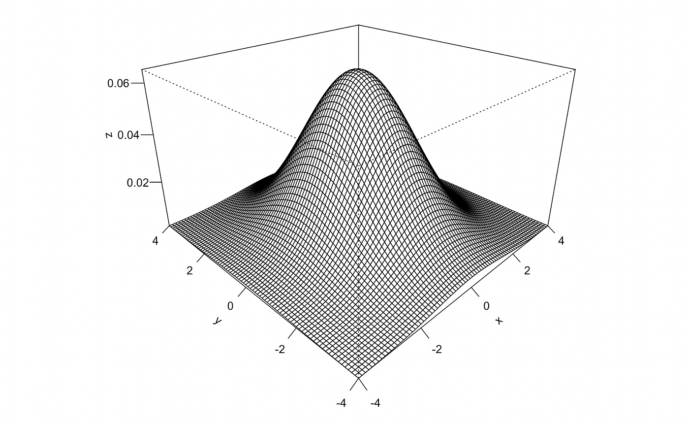
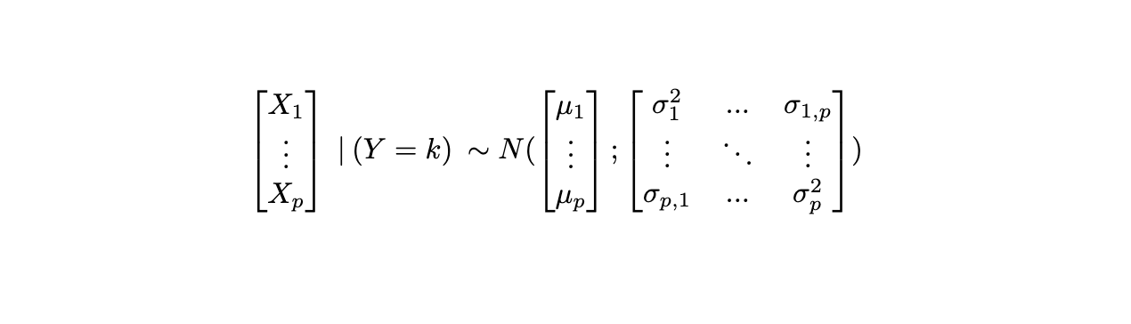
How to decide on an affordable distribution? One clear division arises between predictors which are discrete and steady. All three strategies assume that inside every class,
Predictors have a Gaussian distribution (p=1) or Multivariate Gaussian (p>1).
Therefore, these algorithms can be utilized solely when we now have steady predictors. In truth, Gaussian Naive Bayes is a particular case of normal Naive Bayes, with a Gaussian chance, purpose why I’m evaluating it with LDA and QDA on this publish.
Any longer, we’ll take into account the only case in a position to showcase the variations between the three strategies: two predictors (p=2) and two lessons (Okay=2).
Linear Discriminant Evaluation
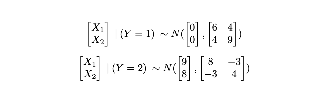
LDA assumes that the covariance matrix throughout lessons is similar.
Which means that predictors in school 1 and sophistication 2 might need totally different means, however their variance and covariance is similar. Which means that the “unfold” and relationship between predictors is similar throughout lessons.

The plot above was generated from distributions for every class of the shape:
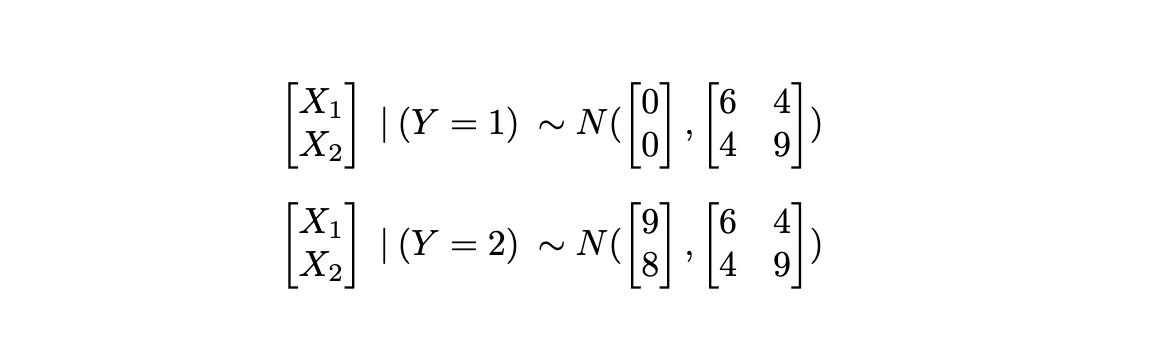
the place we observe that the covariance matrices are the identical. This assumption is cheap if we anticipate the connection between predictors to not change throughout lessons, and if we merely observe a shift within the technique of the distributions.
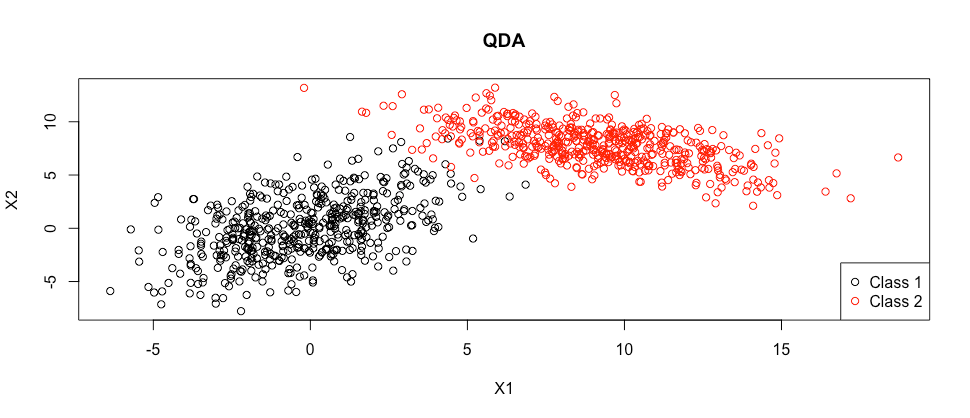
Quadratic Discriminant Evaluation
If we calm down the fixed covariance matrix assumption of LDA, we now have QDA.
QDA doesn’t assume fixed covariance matrix throughout lessons.

The plot above was generated from distributions for every class of the shape:
The place we observe that the 2 distribution are allowed to fluctuate in all of the parameters. This can be a affordable assumption if we anticipate the behaviour and relationships amongst predictors to be very totally different in several lessons.
On this instance, even the course of the connection between the 2 predictors varies from class 1 to class 2, from a constructive covariance of 4, to a adverse covariance of -3.
Gaussian Naive Bayes
GNB is a particular case of the Naive Bayes, the place the predictors are steady and usually distributed inside every class okay. The overall Naive Bayes (and therefore , GNB too) assumes:
Given Y, the predictors X are conditionally impartial.
impartial implies uncorrelated, i.e. have covariance equal to zero.

The plot above was generated from distributions for every class of the shape:
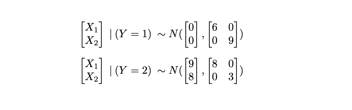
With Naive Bayes we’re assuming there isn’t a relationship between predictors. In actual issues that is not often the case, however it significantly simplifies the issue, as we’ll see within the subsequent part.
Implications of Assumptions
After choosing a mannequin, we estimate the parameters of the within-class distributions to find out the chance of our check statement, and procure the ultimate conditional likelihood we use to categorise it.
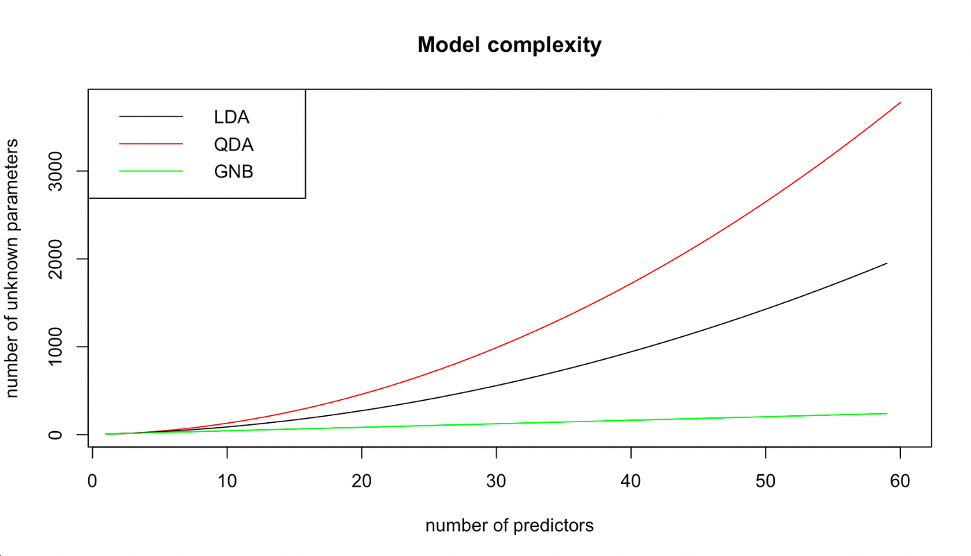
The totally different fashions end in a unique variety of parameters being estimated. Reminder: we now have p predictors and Okay complete lessons. For all fashions we have to estimate technique of the Gaussian distribution of the predictors, that may be totally different in every class. This leads to a base, p*Okay parameters to be estimated for all strategies.
Moreover, if we decide LDA we estimate the variances for all p predictors and covariances for every pair of predictors, leading to

parameters. These are fixed throughout lessons.
For QDA, since they differ in every class, we multiply the variety of parameters for LDA instances Okay, ensuing within the following equation for the estimated variety of parameters:

For GNB, we solely have the variances for all predictors in every class: p*Okay.
It’s straightforward to see the benefit of utilizing GNB for giant values of p and/or Okay. For the regularly occurrent downside of binary classification, i.e. when Okay=2, that is how the mannequin complexity evolves for rising p for the three algorithms.
So What?
From a modelling perspective, realizing what assumptions you’re coping with is essential when making use of a technique. The extra parameters one must estimate, the extra delicate is the ultimate classification to adjustments in our pattern. On the similar time, if the variety of parameters is simply too low, we’ll fail to seize essential variations throughout lessons.
Thanks in your time, I hope it was attention-grabbing.
All pictures until in any other case famous are by the creator.
