Perceive what is keen and lazy execution and the way you need to use lazy execution to optimize your queries
In my earlier article on Polars, I launched you to the Polars DataFrame library that’s far more environment friendly than the Pandas DataFrame.
On this article, I’m going to dive deeper into what makes Polar so quick — lazy analysis. You’ll be taught the distinction between keen execution and lazy analysis/execution.
To know the effectiveness of lazy analysis, it’s helpful to match with how issues are accomplished in Pandas.
For this train, I’m going to make use of the flights.csv file positioned at https://www.kaggle.com/datasets/usdot/flight-delays. This dataset accommodates the flight delays and cancellation particulars for flights within the US in 2015. It was collected and revealed by the DOT’s Bureau of Transportation Statistics.
Licensing — CC0: Public Area (https://creativecommons.org/publicdomain/zero/1.0/).
We will use Pandas to load the flights.csv file, which accommodates 5.8 million rows and 31 columns. Normally, in the event you load this on a machine with restricted reminiscence, Pandas will take a very long time to load it right into a dataframe (if it hundreds in any respect). The next code does the next:
- Load the flights.csv file right into a Pandas DataFrame
- Filters the dataframe to search for these flights in December and whose origin airport is SEA and vacation spot airport is DFW
- Measure the period of time wanted to load the CSV file right into a dataframe and the filtering
import pandas as pd
import timebegin = time.time()df = pd.read_csv('flights.csv')
df = df[(df['MONTH'] == 12) &
(df['ORIGIN_AIRPORT'] == 'SEA') &
(df['DESTINATION_AIRPORT'] == 'DFW')]finish = time.time()
print(finish - begin)
df
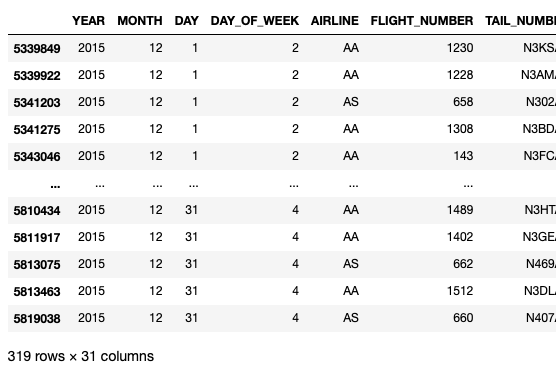
On my M1 Mac with 8GB RAM, the above code snippet took about about 7.74 seconds to load and show the next consequence:
The primary subject with Pandas is that you need to load all of the rows of the dataset into the dataframe earlier than you are able to do any filtering to take away all of the undesirable rows.
When you can load the primary or final n rows of a dataset right into a Pandas DataFrame, to load particular rows (primarily based on sure circumstances) right into a dataframe requires you to load the complete dataset earlier than you’ll be able to carry out the mandatory filtering.
Let’s now use Polars and see if the loading time might be diminished. The next code snippet does the next:
- Load the CSV file utilizing the
read_csv()methodology of the Polars library - Carry out a filter utilizing the
filter()methodology and specify the circumstances for retaining the rows that we would like
import polars as pl
import timebegin = time.time()df = pl.read_csv('flights.csv').filter(
(pl.col('MONTH') == 12) &
(pl.col('ORIGIN_AIRPORT') == 'SEA') &
(pl.col('DESTINATION_AIRPORT') == 'DFW'))finish = time.time()
print(finish - begin)
show(df)
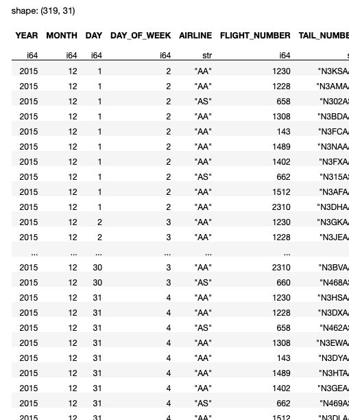
On my pc, the above code snippet took about 3.21 seconds, an enormous enhancements over Pandas:
Now, you will need to know that the read_csv() methodology makes use of keen execution mode, which suggests that it’s going to straight-away load the complete dataset into the dataframe earlier than it performs any filtering. On this side, this block of code that makes use of Polars is just like that of that utilizing Pandas. However you’ll be able to already see that Polars is way sooner than Pandas.
The subsequent enchancment is to switch the read_csv() methodology with one which makes use of lazy execution — scan_csv(). The scan_csv() methodology delays execution till the gather() methodology known as. It analyzes all of the queries proper up until the gather() methodology and tries to optimize the operation. The next code snippet reveals easy methods to use the scan_csv() methodology along with the gather() methodology:
import polars as pl
import timebegin = time.time()
df = pl.scan_csv('flights.csv').filter(
(pl.col('MONTH') == 12) &
(pl.col('ORIGIN_AIRPORT') == 'SEA') &
(pl.col('DESTINATION_AIRPORT') == 'DFW')).gather()
finish = time.time()
print(finish - begin)
show(df)
The
scan_csv()methodology is called an implicit lazy methodology, since by default it makes use of lazy analysis.
For the above code snippet, as an alternative of loading all of the rows into the dataframe, Polars optimizes the question and hundreds solely these rows satisfying the circumstances within the filter() methodology. On my pc, the above code snippet took about 2.67 seconds, an extra discount in processing time in comparison with the earlier code snippet.
Bear in mind earlier on I discussed that the read_csv() methodology makes use of keen execution mode? What if you wish to use lazy execution mode on it? Effectively, you’ll be able to merely name the lazy() methodology on it after which finish the complete expression utilizing the gather() methodology, like this:
import polars as pl
import timebegin = time.time()
df = pl.read_csv('flights.csv').lazy().filter(
(pl.col('MONTH') == 12) &
(pl.col('ORIGIN_AIRPORT') == 'SEA') &
(pl.col('DESTINATION_AIRPORT') == 'DFW')).gather()
finish = time.time()
print(finish - begin)
show(df)
By utilizing the lazy() methodology, you might be instructing Polars to carry on the execution and as an alternative optimize all of the queries proper as much as the gather() methodology. The gather() methodology begins the execution and collects the consequence right into a dataframe. Primarily, this methodology instructs Polars to eagerly execute the question.
Let’s now break down a question and see how Polars truly works. First, let’s use the scan_csv() methodology and see what it returns:
pl.scan_csv('titanic_train.csv')
Supply of Knowledge: The info supply for this text is from https://www.kaggle.com/datasets/tedllh/titanic-train.
Licensing — Database Contents License (DbCL) v1.0 https://opendatacommons.org/licenses/dbcl/1-0/
The above assertion returns a “polars.internals.lazy_frame.LazyFrame” object. In Jupyter Pocket book, it is going to present the next execution graph (I’ll speak extra about this as we go alongside):
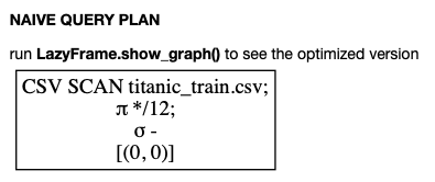
The execution graph reveals the sequence by which Polars will execute your question.
The LazyFrame object that’s returned represents the question that you’ve got formulated, however not but executed. To execute the question, it is advisable to use the gather() methodology:
pl.scan_csv('titanic_train.csv').gather()
You can even enclose the question utilizing a pair of parentheses and assign it to a variable. To execute the question, you merely name the gather() methodology of the question, like this:
q = (
pl.scan_csv('titanic_train.csv')
)
q.gather()
The benefit of enclosing your queries in a pair of parentheses is that it means that you can chain a number of queries and put them in separate traces, thereby drastically enhancing readability.
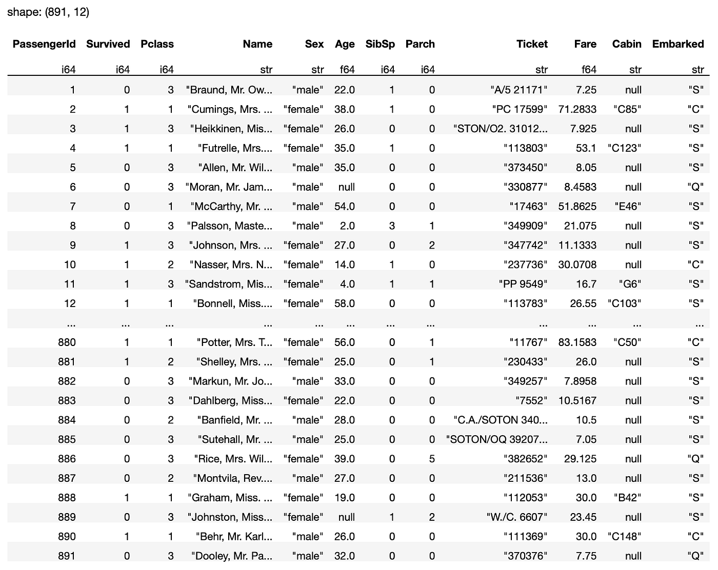
The above code snippet reveals the next output:
For debugging functions, typically it’s helpful to only return a number of rows to look at the output, and so you need to use the fetch() methodology to return the primary n rows:
q.fetch(5)
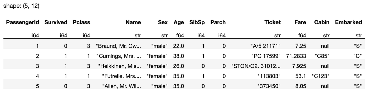
The above assertion returns the primary 5 rows of the consequence:
You possibly can chain the varied strategies in a single question:
q = (
pl.scan_csv('titanic_train.csv')
    .choose(['Survived','Age'])
.filter(
pl.col('Age') > 18
)
)
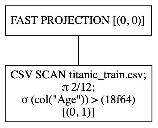
The show_graph() methodology shows the execution graph that you’ve got seen earlier, with a parameter to point if you wish to see the optimized graph:
q.show_graph(optimized=True)
The above assertion reveals the next execution graph. You possibly can see that the filtering primarily based on the Age column is completed collectively in the course of the loading of the CSV file:
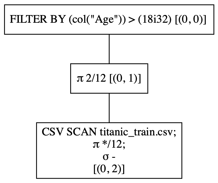
In distinction, let’s see how the execution move will appear like if the queries are executed in keen mode (i.e. non-optimized):
q.show_graph(optimized=False)
As you’ll be able to see from the output under, the CSV file is first loaded, adopted by the collection of the 2 columns, and at last the filtering is carried out:
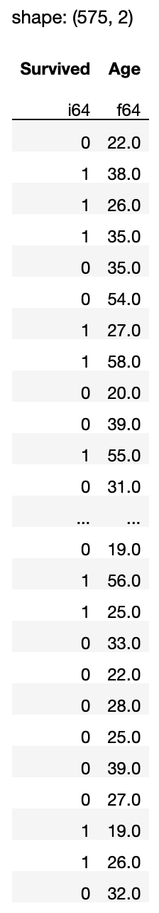
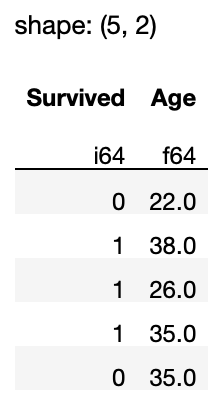
To execute the question, name the gather() methodology:
q.gather()
The next output shall be proven:
If you happen to solely need the primary 5 rows, name the fetch() methodology:
q.fetch(5)
I hope you now have a greater thought of how lazy execution works in Polars and easy methods to allow it even for queries that helps solely keen execution. Displaying the execution graph makes it simpler so that you can perceive how your queries are being optimized. Within the subsequent few articles, I’ll proceed my dialogue on the Polars DataFrame and the varied methods to govern them. If there may be any explicit matter that you really want me to give attention to, depart me a remark!
