The Grammar of Graphics or the way to do ggplot-style plotting in Julia | by Roland Schätzle | Aug, 2022

Introduction to a comparability of Julia graphics packages for statistical plotting

The Grammar of Graphics (GoG) is an idea that has been developed by Leland Wilkinson (The Grammar of Graphics, Springer, 1999) and refined by Hadley Wickham (A Layered Grammar of Graphics, Journal of Computational and Graphical Statistics, vol. 19, no. 1, pp. 3–28, 2010; pdf).

Its essential concept is that each statistical plot could be created by a mixture of some fundamental constructing blocks (or mechanisms). This permits

• a easy and concise definition of a visualization
• a straightforward adaptation of a visualization by exchanging solely the constructing blocks that are affected in a modular approach
• reusable specs (the identical visualization can e.g. be utilized to completely different knowledge)

Wickham confirmed that this idea just isn’t solely a pleasant concept. He carried out it within the R-package ggplot2 which turned fairly well-liked. A number of GoG-implementations are additionally accessible for the Julia programming language.

On this article I’ll first clarify the fundamental ideas and concepts of the Grammar of Graphics. In follow-up articles I’ll then current the next 4 Julia graphics packages that are based mostly (utterly or partially) on the GoG:

With a view to enable you a 1:1-comparison of those Julia packages, I’ll use the identical instance plots and the identical underlying knowledge for every article. Within the second a part of this text, I’ll current the information used for the examples, so I don’t should repeat that in every of the follow-up articles.

Within the subsequent sections I’ll clarify the fundamental concepts of “The Grammar of Graphics” by Wilkinson in addition to “A Layered Grammar of Graphics” by Wickham. I gained’t go into each element and in features the place each ideas differ, I’ll intentionally decide one and provides a fairly “unified” view.

For the code examples, I’m utilizing Julia’s Gadfly-package (vers. 1.3.4 & Julia 1.7.3).

The primary elements

The primary constructing blocks for a visualization are

Knowledge
Essentially the most acquainted of those three ideas might be knowledge. We assume right here, that knowledge is available in tabular kind (like a database desk). For a visualization it’s vital to tell apart between numerical and categorical knowledge.

Right here we have now e.g. the stock checklist of a fruit seller:

Row │ amount  fruit   value 
────────────────────────────────
1  │    3     apples   2.5
2  │   20     oranges  3.9
3  │    8     bananas  1.9

It consists of the three variables amount, fruit and value. fruit is a categorical variable whereas the opposite two variables are numerical.

Aesthetics
To visualise an information variable, it’s mapped to a number of aesthetics.

Numerical variables could be mapped e.g. to a

• place on the x-, y- or z-axis
• dimension

Categorical variables could be mapped e.g. to a

Geometry
Other than knowledge variables and aesthetics we want not less than a geometry to specify a whole visualization. The geometry tells us principally which sort of diagram we wish. Some examples are:

• line (= line diagram)
• level (= scatter plot)
• bar (= bar plot)

Fundamental examples

Now we have now sufficient data to construct our first visualizations based mostly on the Grammar of Graphics. For the code examples utilizing the Gadfly-package we assume, that the stock desk above is in a variable named stock of sort DataFrame.

First we wish to see how the portions are distributed by value. Relying on the geometry chosen, we get both a scatter plot or a line diagram:

• Map value to the x-axis, amount to the y-axis
  utilizing a level geometry
  In Gadfly: plot(stock, x = :value, y = :amount, Geom.level)

• Map value to the x-axis, amount to the y-axis
  utilizing a line geometry
  In Gadfly: plot(stock, x = :value, y = :amount, Geom.line)

Within the subsequent step we wish moreover see, which fruits are concerned. So we have now to map fruit to an appropriate aesthetic too. Within the following two examples first a form is used after which a colour.

• Map value to the x-axis, amount to the y-axis, fruit to a form
  utilizing a level geometry
  In Gadfly: plot(stock, x = :value, y = :amount, form = :fruit, Geom.level)

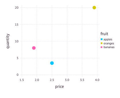
• Map value to the x-axis, amount to the y-axis, fruit to a colour
  utilizing a level geometry
  In Gadfly: plot(stock, x = :value, y = :amount, colour = :fruit, Geom.level)

Additionally it is potential to map one variable to a number of aesthetics. We are able to e.g. map fruit to form in addition to colour.

• Map value to the x-axis, amount to the y-axis,
  fruit to a form, fruit to a colour,
  utilizing a level geometry
  In Gadfly: plot(stock, x = :value, y = :amount,
form = :fruit, colour = :fruit, Geom.level)

Utilizing a bar geometry we will plot a statistics of the portions in inventory. Right here we map a categorical variable (fruit) to positions on the x-axis.

• Map fruit to the x-axis, amount to the y-axis utilizing a bar geometry
  In Gadfly: plot(stock, x = :fruit, y = :amount, Geom.bar)

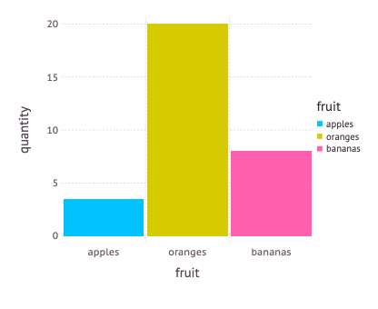
If we map fruit additionally to a colour, the bars shall be displayed in several colours:

• Map fruit to the x-axis, amount to the y-axis, fruit to a colour
  utilizing a bar geometry
  In Gadfly: plot(stock, x = :fruit, y = :amount, colour = :fruit, Geom.bar)

These fundamental examples present properly how a visualization could be specified utilizing just a few easy constructing blocks, thus making up a strong visualization language.

They present additionally that these specs allow a graphics bundle to derive significant defaults for quite a lot of features of a visualization which aren’t given explicitly.

All of the examples had

• significant scales for the x- and y-axis (usually utilizing a barely bigger interval than that of the information variable given)
• along with acceptable ticks and axis labeling
• in addition to a descriptive label (merely utilizing the variable identify)

Some examples even had an mechanically generated legend. That is potential as a result of a legend is solely the inverse operate of an information mapping to an aesthetic. If we e.g. map the variable fruit to a colour, then the corresponding legend is the reverse mapping from colour to fruit.

Extra elements

To be sincere, we want just a few extra parts than simply knowledge, aesthetics and a geometry for a whole visualization.

Scale
With a view to map numerical variables e.g. to positional aesthetics (just like the positions on the x- or y-axis), we want additionally a scale which maps the information items to bodily items (e.g. of the display screen, a window or an internet web page).

Within the examples above, a linear scale was utilized by default. However we might additionally alternate it e.g. with a logarithmic scale.

It’s additionally potential to map a numerical variable to a colour. Then a steady colour scale is used for that mapping as we will see within the following instance:

• Map value to the x-axis, amount to the y-axis, amount to a colour
  utilizing a level geometry
  In Gadfly: plot(stock, x = :value, y = :amount,
colour = :amount, Geom.level)

Coordinate system
Carefully associated to a scale is the idea of a coordinate system, which defines how positional values are mapped onto the plotting aircraft. Within the examples above, the Cartesian coordinate system has been utilized by default. Different prospects are polar or barycentric coordinate methods or the assorted methods that are used for map projections.

It’s an fascinating facet that we will produce several types of diagrams from the identical knowledge and aesthetics mappings, simply by altering the coordinate system: E.g. a bar plot relies on the Cartesian coordinate system. If we substitute that with a polar system, we get a Coxcomb chart, as the next instance from R for Knowledge Science (by Hadley Wickham and Garret Grolemund, O’Reilly, 2017) reveals.

Conclusions

With these two further ideas we have now now a whole image of the fundamental GoG. On this brief article I might in fact solely current a subset of all potential aesthetics and graphics and there are extra parts to the GoG like statistics and sides. However what we have now seen to this point is the core of the Grammar of Graphics and must be sufficient to know the primary concepts.

Let’s now swap to the comparability of various Julia graphics packages which I’ll current in a number of follow-up articles. As type of a preparation I’ll now current the information used for various instance plots (that are impressed by the YouTube tutorial Julia Evaluation for Rookies from the channel julia for gifted amateurs) inside these follow-up articles and provides an outlook on what kinds of diagrams I’ll use for the comparability.

Nations by GDP

The premise of the information used for the plotting examples is a listing of all international locations and their GDP and inhabitants dimension for the years 2018 and 2019. It’s from this Wikipedia-page (which obtained the information from a database of the IMF and the United Nations). The information can also be accessible in CSV-format from my GitHub-repository.

The columns of the checklist have the next that means:

• ID: distinctive identifier
• Area: the continent the place the nation is situated
• Subregion: every continent is split into a number of subregions
• Pop2018: inhabitants of the nation in 2018 [million people]
• Pop2019: inhabitants of the nation in 2019 [million people]
• PopChangeAbs: change in inhabitants from 2018 to 2019 in absolute numbers [million people]
• PopChangePct: like PopChangeAbs however as a proportion [%]
• GDP: gross home product of the nation in 2019 [million USD]
• GDPperCapita: GDP divided by the variety of individuals dwelling within the nation [USD/person]; this column just isn’t within the supply file, however shall be computed (see under)

The file is downloaded and transformed to a DataFrame utilizing the next Julia code:

Line 7 computes the brand new column GDPperCapita talked about above and provides it to the international locations-DataFrame.

Aggregated knowledge

The detailed checklist which has one row per nation (in 210 rows) shall be grouped and aggregated on two ranges (utilizing DataFrame-functions):

Stage 1 — Areas: The next code teams the checklist by Area (i.e. continent) omitting the columns Nation and Subregion (utilizing a nested choose) in line 1 after which creates an aggregation summing up all numerical columns (strains 2–5).

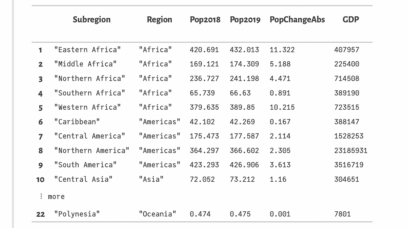
Stage 2 — Subregions: The identical operations are utilized on the subregion degree in strains 7–11. First the international locations are grouped by Subregion omitting column Nation (line 7) after which an aggregation is created on that knowledge; once more summing up all numerical columns. Apart from, the identify of the area is picked from every subgroup (:Area => first )

This ensuing DataFrames regions_cum and subregions_cum look as follows:

Abstract

The DataFrames international locations, subregions_cum and regions_cum are the premise for the plotting examples within the forthcoming articles concerning the completely different Julia graphics packages. In these articles we’ll see the way to create

• bar plots
• scatter plots
• histograms
• field plots and violin plots

in every of those graphics packages.

The primary article will current Gadfly. So keep tuned!