
An instance in MATLAB

A Gaussian distribution is without doubt one of the many statistical distributions that may describe information units, and it’s a essential one as many real-life processes comply with this distribution. Examples of gaussian distributions embrace monetary returns and top in populations.
On this instance, we’ll artificially generate a pattern information out of a Gaussian distribution, plot it in opposition to the theoretical Gaussian distribution curve and later apply the Kolmogorov-Smirnov check if the info set is a part of a gaussian distribution or not — which on this case clearly is, because it has been generated from a traditional distribution — .
On this instance, we’ll use MATLAB, however after all, there are one-to-one equivalences utilizing numpy and Matplotlib. The Gaussian mannequin chance density operate exhibits how a lot chance has sure values over others.

Step one is to create the Gaussian distribution mannequin. On this case, we’ll use mu (μ) equal to 2 and sigma (σ) equal to 1. μ represents the imply worth, and σ represents the place 68% of the info is positioned. Utilizing 2 σ will present the place 95% of the info is positioned. Sigma (σ) is measured from the imply (μ) and represents how far or shut information is respect to the imply.
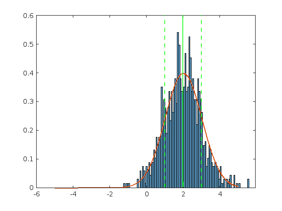
As a second step we’ll make two plots, one plots the pattern information and the opposite plots the histogram of the pattern information and the theoretical Gaussian curve.
This creates each plots:
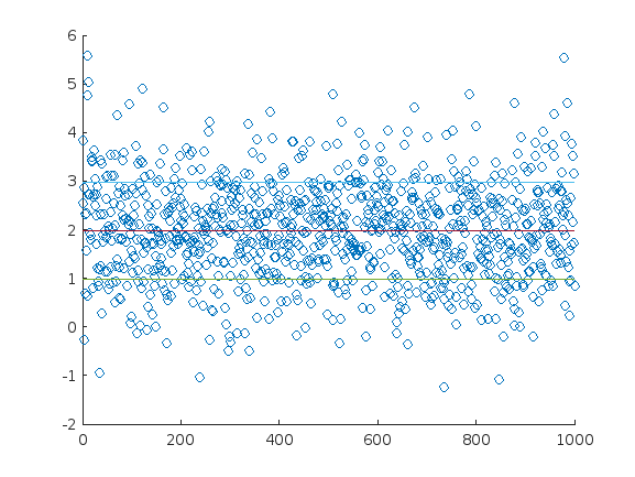

Whereas plotting the info factors we will see how they’re concentrated round μ and that a lot of the information (68%) is contained inside μ-σ and μ+σ.
Within the second chart, we see how the theoretical gaussian curve has a a lot smaller scale than our information set, this is because of we have now to scale the world of our information set to 1. Matlab can do this routinely for us through a normalisation parameter:
On this instance, we have now generated the info artificially from a gaussian distribution mannequin. That clearly implies that the info is Gaussian. Whereas typically that’s supposed (we would need a dataset that comes straight forward from a traditional distribution) more often than not we’ll simply face information which appears gaussian in nature and we wish to validate that assumption.
There are a number of strategies to check if an information set is gaussian or not. One among them is the Kolmogorov-Smirnov check which evaluates the null speculation of information being Gaussian.
The default Kolmogorov-Smirnov check is predicated on an information pattern with a imply 0 and a sigma 1. So if we apply the check to our dataset we’ll return that the dataset will not be gaussian. In actuality, it’s about specifying the imply and the sigma.
If we subtract the anticipated imply and divide it by the variance, we will then apply the check usually.
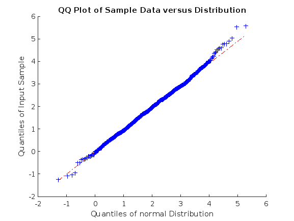
The Q-Q plot is a visible solution to test if an information set is gaussian or not. In MATLAB there’s the choice to specify a distribution or not, though each plots appear the identical the appropriate one is the second (the one which makes use of the distribution that we created) because it generates an correct axis (imply and sigma).
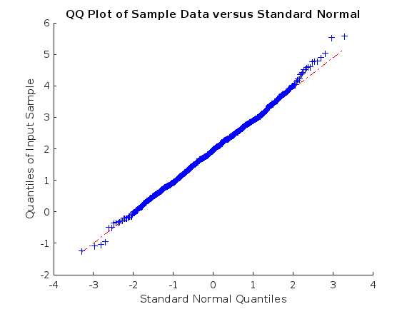
Observe how the second diagram is centered round our distribution imply:
Quantile-to-quantile plots are a straightforward and visible solution to present how a dataset matches right into a gaussian mannequin.
Skewness and Kurtosis are two well-known measures that may be utilized to Gaussian distributions.
Skewness measures the asymmetry across the imply, a numerical worth that can let you know if there are extra values on the proper of the imply or the left. An ideal symmetrical gaussian will result in a skewness with a price of 0. Skewness values lower than 0.5 are roughly symmetrical, values between 0.5 and 1 are reasonably asymmetrical and values above 1 are largely asymmetrical. The particular thresholds will rely in your particular mannequin although.
Kurtosis is a measure of how excessive the tail of the distribution is, and it’s typically known as a measure of the form of the height of the distribution, though that interpretation is discredited. Subsequently, it may be used as a function to find out how far the outliers go in a specific distribution.
Each measures are simple to acquire in Matlab. For the Skewness, utilizing 0 as an extra parameter will subtract the imply. Particulars for each instructions will be discovered within the Matlab documentation.
The Gaussian distribution is probably going crucial statistical distribution in lots of disciplines, and it’s usually a requirement for the info to use many transformations and mathematical strategies. Realizing easy methods to create Gaussian datasets, easy methods to interpret its chance distribution operate, easy methods to normalise the info and easy methods to validate if a dataset is Gaussian or not are all fundamental expertise that prior to later might be required in information science.
