The Bayesian Bootstrap. A brief information to a easy and highly effective… | by Matteo Courthoud | Aug, 2022

CAUSAL DATA SCIENCE

A brief information to a easy and highly effective various to the bootstrap

In causal inference we don’t want simply to compute therapy results, we additionally need to do inference (duh!). In some instances, it’s very simple to compute the (asymptotic) distribution of an estimator, because of the central restrict theorem. That is the case when computing the typical therapy impact in AB assessments or randomized managed trials, for instance. Nonetheless, in different settings, inference is extra sophisticated, when the article of curiosity will not be a sum or a median, as, for instance, with the median therapy impact. In these instances, we can not depend on the central restrict theorem. What can we do then?

The bootstrap is the usual reply in information science. It’s a very highly effective process to estimate the distribution of an estimator, while not having any data of the info producing course of. Additionally it is very intuitive and easy to implement: simply re-sample your information with substitute a whole lot of instances and compute your estimator throughout samples.

Can we do higher? The reply is sure! The Bayesian Bootstrap is a strong process that in a whole lot of settings performs higher than the bootstrap. Particularly, it’s often sooner, may give tighter confidence intervals, and avoids a whole lot of nook instances. On this article, we’re going to discover this straightforward however highly effective process extra intimately.

The bootstrap is a process to compute the properties of an estimator by random re-sampling with substitute from the info. It was first launched by Efron (1979) and it’s now a regular inference process in information science. The process may be very easy and consists of the next steps.

Suppose you have got entry to an i.i.d. pattern {Xᵢ}ᵢⁿ and also you need to compute a statistic θ utilizing an estimator θ̂(X). You’ll be able to approximate the distribution of θ̂ as follows.

1. Pattern n observations with substitute {X̃ᵢ}ᵢⁿ out of your pattern {Xᵢ}ᵢⁿ.
2. Compute the estimator θ̂-bootstrap(X̃).
3. Repeat steps 1 and a couple of numerous instances.

The distribution of θ̂-bootstrap is an efficient approximation of the distribution of θ̂.

Why is the bootstrap so highly effective?

Initially, it’s simple to implement. It doesn’t require you to do something greater than what you had been already doing: estimating θ. You simply must do it a whole lot of instances. Certainly, the primary drawback of the bootstrap is its computational price. In case your estimating process is gradual, bootstrapping turns into prohibitive.

Second, the bootstrap makes no distributional assumptions. It solely assumes that your pattern is consultant of the inhabitants, and observations are unbiased of one another. This assumption could be violated when observations are tightly related with one another, reminiscent of when finding out social networks or market interactions.

Is bootstrap simply weighting?

In the long run, after we re-sample, what we’re doing is assigning integer weights to our observations, such that their sum provides as much as the pattern dimension n. Such distribution is the multinomial distribution.

Let’s take a look at what a multinomial distribution seems to be like by drawing a pattern of dimension 10.000. I import a set of ordinary libraries and capabilities from src.utils. I import the code from Deepnote, a Jupyter-like web-based collaborative pocket book setting. For our function, Deepnote may be very useful as a result of it permits me not solely to incorporate code but additionally output, like information and tables.

Initially, we examine that certainly the weights sum as much as 1000, or equivalently, that we generated a re-sample of the identical dimension of the info.

We are able to now plot the distribution of weights.

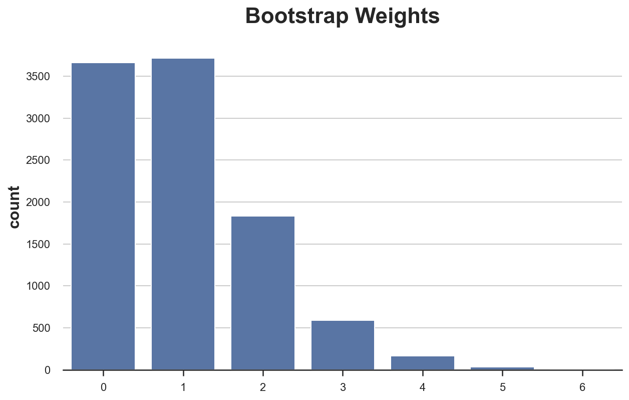
As we will see, round 3600 observations bought zero weight, whereas a few observations bought a weight of 6. Or equivalently, round 3600 observations didn’t get re-sampled, whereas a few observations had been sampled as many as 6 instances.

Now you might need a spontaneous query: why not use steady weights as an alternative of discrete ones?

Superb query! The Bayesian Bootstrap is the reply.

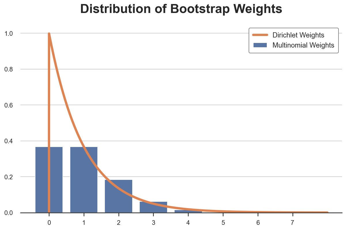
The Bayesian bootstrap was launched by Rubin (1981) and it’s primarily based on a quite simple concept: why not draw a smoother distribution of weights? The continual equal of the multinomial distribution is the Dirichlet distribution. Under I plot the likelihood distribution of Multinomial and Dirichelet weights for a single remark (they’re Poisson and Gamma distributed, respectively).

The Bayesian Bootstrap has many benefits.

• The primary and most intuitive one is that it delivers estimates which can be far more easy than the conventional bootstrap, due to its steady weighting scheme.
• Furthermore, the continual weighting scheme prevents nook instances from rising, since no remark will ever obtain zero weight. For instance, in linear regression, no downside of collinearity emerges, if there wasn’t one within the authentic pattern.
• Lastly, being a Bayesian methodology, we acquire interpretation: the estimated distribution of the estimator will be interpreted because the posterior distribution with an uninformative prior.

Let’s now draw a set a Dirichlet weights.

The weights naturally sum to (roughly) 1, so now we have to scale them by an element N.

As earlier than, we will plot the distribution of weights, with the distinction that now now we have steady weights, so now we have to approximate the distribution.

As you might need observed, the Dirichlet distribution has a parameter α that now we have set to 1 for all observations. What does it do?

The α parameter primarily governs each absolutely the and relative likelihood of being sampled. Rising α for all observations makes the distribution much less skewed so that each one observations have a extra related weight. For α→∞, all observations obtain the identical weight and we’re again to the unique pattern.

How ought to we choose the worth of α? Shao and Tu (1995) recommend the next.

The distribution of the random weight vector doesn’t must be restricted to the Diri(l, … , 1). Later investigations discovered that the weights having a scaled Diri(4, … ,4) distribution give higher approximations (Tu and Zheng, 1987)

Let’s take a look at how a Dirichlet distribution with α=4 for all observations compares to our earlier distribution with α=1 for all observations.

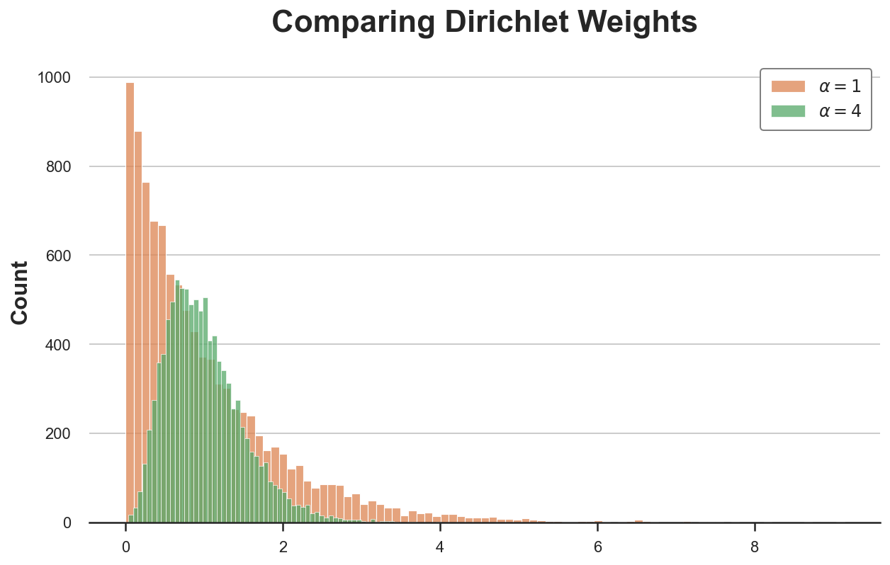
The brand new distribution is way much less skewed and extra concentrated across the common worth of 1.

Let’s take a look at a few examples, the place we evaluate each inference procedures.

Imply of a Skewed Distribution

First, let’s take a look at one of many easiest and most typical estimators: the pattern imply. First, let’s draw 100 observations from a Pareto distribution.

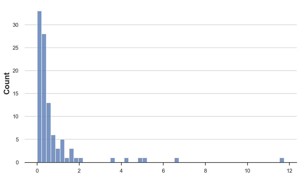
This distribution may be very skewed, with a few observations taking a lot greater values than the typical.

First, let’s compute the traditional bootstrap estimator for one re-sample.

Then, let’s write the Bayesian bootstrap for one set of random weights.

We are able to now implement any bootstrap process. I exploit the joblib library to parallelize the computation.

Lastly, let’s write a operate that compares the outcomes.

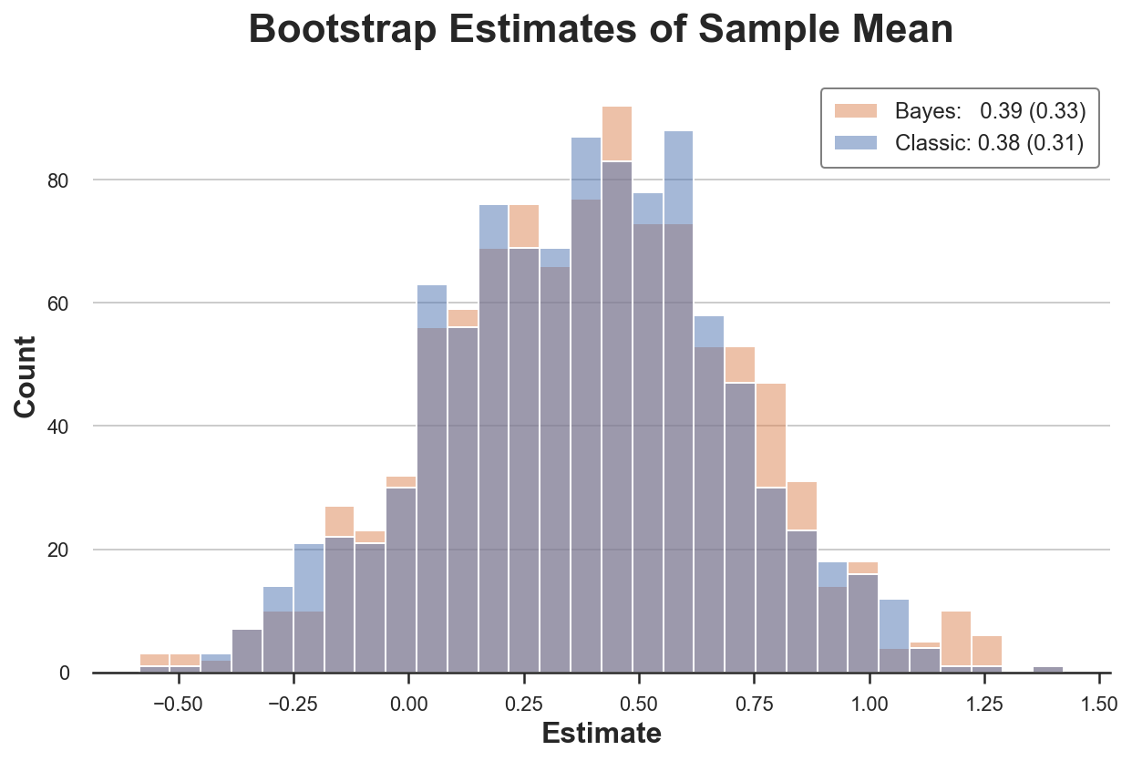
On this setting, each procedures give a really related reply. The 2 distributions are very shut, and in addition the estimated imply and commonplace deviation of the estimator is nearly the identical, irrespectively to the bootstrap process.

Which bootstrap process is sooner?

The Bayesian bootstrap is quicker than the classical bootstrap in 99% of the simulations and by a powerful 75%!

No Weighting? No Drawback

What if now we have an estimator that doesn’t settle for weights, such because the median? We are able to do two-level sampling: first we pattern the weights after which we pattern observations in response to the weights.

On this setting, the Bayesian Bootstrap can also be extra exact than the classical bootstrap, due to the denser weight distribution with α=4.

Logistic Regression with Uncommon Consequence

Let’s now discover the primary of two settings during which the classical bootstrap would possibly fall into nook instances. Suppose we noticed a characteristic x, usually distributed, and a binary end result y. We have an interest within the relationship between the 2 variables.

On this pattern, we observe a optimistic end result solely in 10 observations out of 100.

Because the end result is binary, we match a logistic regression mannequin.

We get a degree estimate of -23 with a really tight confidence interval.

Can we bootstrap the distribution of our estimator? Let’s attempt to compute the logistic regression coefficient over 1000 bootstrap samples.

For five samples out of 1000, we’re unable to compute the estimate. This is able to not have occurred with the Bayesian bootstrap.

This would possibly appear to be an innocuous problem on this case: we will simply drop these observations. Let’s conclude with a way more harmful instance.

Regression with few Handled Items

Suppose we noticed a binary characteristic x and a steady end result y. We’re once more within the relationship between the 2 variables.

Let’s evaluate the 2 bootstrap estimators of the regression coefficient of y on x.

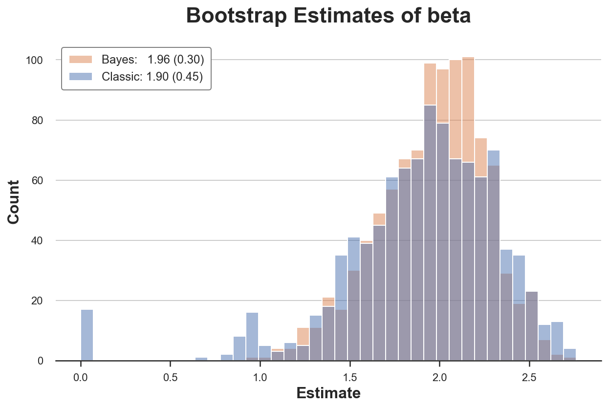
The traditional bootstrap process estimates a 50% bigger variance than our estimator. Why? If we glance extra carefully, we see that in virtually 20 re-samples, we get a really uncommon estimate of zero! Why?

The issue is that in some samples we’d not have any observations with x=1. Due to this fact, in these re-samples, the estimated coefficient is zero. This doesn’t occur with the Bayesian bootstrap, because it doesn’t drop any remark (all observations at all times get a optimistic weight).

The problematic half right here is that we aren’t getting any error message or warning. This bias may be very sneaky and will simply go unnoticed!

On this article, now we have seen a strong extension of the bootstrap: the Bayesian bootstrap. The important thing concept is that at any time when our estimator will be expressed as a weighted estimator, the bootstrap is equal to random weighting with multinomial weights. The Bayesian bootstrap is equal to weighting with Dirichlet weights, the continual equal of the multinomial distribution. Having steady weights avoids nook instances and might generate a smoother distribution of the estimator.

This text was impressed by the next tweet by Brown College professor Peter Hull.

Thanks for studying!

I actually respect it! 🤗 When you appreciated the publish and wish to see extra, contemplate following me. I publish as soon as every week on matters associated to causal inference and information evaluation. I attempt to hold my posts easy however exact, at all times offering code, examples, and simulations.

Additionally, a small disclaimer: I write to study so errors are the norm, though I strive my finest. Please, once you spot them, let me know. I additionally respect recommendations on new matters!

References

[1] B. Efron Bootstrap Strategies: One other Have a look at the Jackknife (1979), The Annals of Statistics.
[2] D. Rubin, The Bayesian Bootstrap (1981), The Annals of Statistics.
[3] A. Lo, A Massive Pattern Research of the Bayesian Bootstrap (1987), The Annals of Statistics.
[4] J. Shao, D. Tu, Jacknife and Bootstrap (1995), Springer.
Code
You will discover the unique Jupyter Pocket book right here: