This text will undergo how you can use the favored XGBoost library for Studying-to-rank(LTR) issues
The most typical use instances of LTR are Search Engines and Recommender Techniques. The final word aim of rating is to order gadgets in a significant order.
This text will use the favored XGBoost library for film suggestions.
When beginning engaged on LTR, my first query was, what’s the distinction between conventional machine studying and rating issues? So that is what I discovered. Every occasion has a goal class or worth in conventional machine studying issues. For instance, In case you are working with a churn prediction drawback, you have got the characteristic set for every buyer and related courses. Likewise, our output could be a buyer id and predicted class or likelihood rating. However in LTR, we do not have a single class or worth for every occasion. As an alternative, we’ve a number of gadgets and their floor reality worth per occasion, and our output would be the optimum ordering of these gadgets. For instance, If we’ve a consumer’s previous interplay with gadgets, Our intention is to construct a mannequin able to predicting optimum user-item pairs.
Now it is time to get into the coding half. For simplicity, I will use the movielens¹ small dataset. You possibly can obtain the dataset utilizing the under hyperlink.
Let’s load the dataset and do primary preprocessing on the dataset.
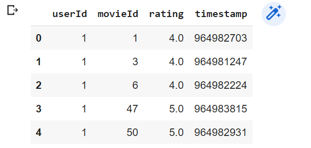
On this dataset, we’ve 100,000 scores and three,600 tag purposes utilized to 9,000 motion pictures by 600 customers.
Let’s shortly take a look at the ranking column.
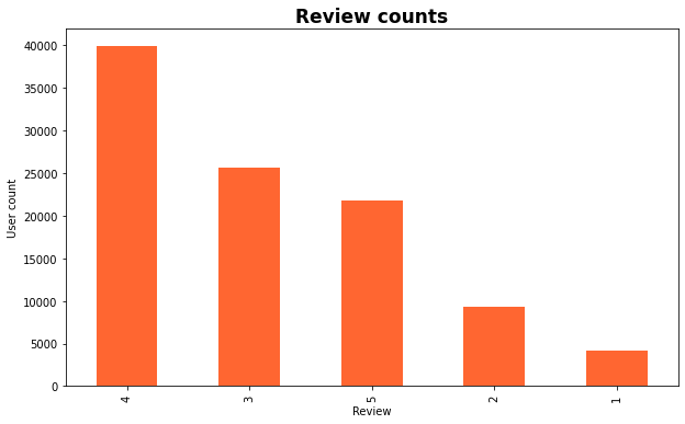


After wanting on the above plots, I added a time-based, day-based characteristic for the modeling. So, I’ll create user-level and item-level options. For instance, for some film “X”, I get a complete variety of customers interacted with, 5,4,3,2, and 1-star critiques acquired. Additionally, I’m including acquired critiques each day and acquired critiques after 5 PM.
Let’s cut up the dataset into prepare and take a look at units. I will use the previous as coaching, and the newest knowledge will use to guage the mannequin.
Now it is time to create mannequin inputs. For the reason that rating mannequin differs from conventional supervised fashions, we’ve to enter extra data into the mannequin. Now time to create the mannequin. We are going to use xgboost, XGBRanker. Let’s concentrate on it is.match methodology. Under is the docstring for XGBRanker().match().
Signature: mannequin.match(X, y, group, sample_weight=None, eval_set=None, sample_weight_eval_set=None, eval_group=None, eval_metric=None, early_stopping_rounds=None, verbose=False, xgb_model=None, callbacks=None)
Docstring: Match the gradient boosting mannequinParameters
X : array_like Characteristic matrix
y : array_like Labels
group : array_like group dimension of coaching knowledge
sample_weight : array_like group weights
.. notice:: Weights are per-group for rating duties In rating process, one weight is assigned to every group (not every knowledge level). It is because we solely care in regards to the relative ordering of knowledge factors inside every group, so it doesn’t make sense to assign weights to particular person knowledge factors.
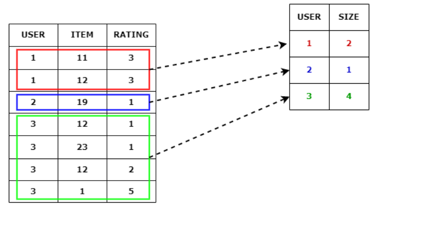
As per the under docstring, we’ve to enter group for each coaching and take a look at samples. So the query is how you can create a bunch array in rating fashions. I noticed many individuals who struggled to grasp this group parameter.
In easy phrases, the group parameter signifies the variety of interactions per consumer. As per the under snippet, you’ll be able to see consumer primary has interacted with two gadgets (11 & 12). Therefore, the consumer 1 group dimension is 2. Moreover, group size ought to equal the variety of distinctive customers within the dataset, and the sum of group dimension ought to equal the overall variety of data within the dataset. In under instance group parameter is [2,1,4].
Let’s create mannequin inputs. We are able to use the under code for that.
Now we’ve prepare and take a look at inputs to feed into the mannequin. It is time to prepare and consider the mannequin. Earlier than doing that, I’ve a number of terminologies to clarify for the article’s completeness.
When mannequin constructing, measuring the standard of the predictions is crucial. What are the obtainable measurements for evaluating advice fashions? There are few, however the commonest measures are Normalized Discounted Cumulative Acquire (NDCG) and Imply Common Precision (MAP). Right here I’ll use NDCG as an analysis metric. NDCG is the improved model of CG (Cumulative Acquire). In CG, recommending an order doesn’t matter. In case your outcomes include related gadgets in any order, this offers you the next worth, indicating our predictions are good. However in the true world, it is not the case. We must always prioritize related gadgets when recommending. To realize this, we must always penalize when low relevance gadgets seem earlier within the outcomes. That’s what DCG does. However nonetheless, DCG suffers when totally different customers have a unique set of merchandise/interplay counts. That is the place Normalized Discounted Cumulative Acquire (NDCG) comes into play. It’ll convey normalization to the DCG metric.
Now we will transfer to the mannequin half.
Now we will generate some predictions.
Listed here are some generated predictions.

It is at all times good to guage the protection of your recommender mannequin. Utilizing the protection metric, you’ll be able to verify the proportion of coaching merchandise within the take a look at set. The extra protection higher the mannequin. In some instances mannequin tries to foretell common retailers to maximise NDCG and MAP@ok. I had this subject once I was engaged on starpoints product suggestions. When we’ve doubts about our analysis metric, we will shortly verify the protection of our mannequin. On this mannequin, I obtained round 2% protection. Signifies our mannequin ought to enhance additional.
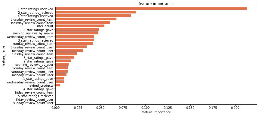
Moreover, we will plot characteristic significance as follows.
On this article, we went via the fundamentals of learning-to-rank issues, how we will mannequin rank issues, and some ideas associated to evaluating advice fashions. Though this text exhibits how we will use xgboost for product rating issues, we will additionally use this strategy for different rating issues.
References
1 [Grouplence ]
F. Maxwell Harper and Joseph A. Konstan. 2015. The MovieLens Datasets: Historical past and Context. ACM Transactions on Interactive Clever Techniques (TiiS) 5, 4: 19:1–19:19. https://doi.org/10.1145/2827872
Thanks for studying. Join with me on LinkedIn.
