Be taught the mathematics and strategies behind the libraries you utilize every day as a knowledge scientist

To extra formally handle the necessity for a statistics lecture collection on Medium, I’ve began to create a collection of statistics boot camps, as seen within the title above. These will construct on each other and as such will probably be numbered accordingly. The motivation for doing so is to democratize the information of statistics in a ground-up vogue to handle the necessity for extra formal statistics coaching within the knowledge science neighborhood. These will start easy and increase upwards and outwards, with workout routines and labored examples alongside the best way. My private philosophy with regards to engineering, coding, and statistics is that in case you perceive the mathematics and the strategies, the abstraction now seen utilizing a large number of libraries falls away and means that you can be a producer, not solely a client of knowledge. Many aspects of those will probably be a evaluation for some learners/readers, nevertheless having a complete understanding and a useful resource to consult with is essential. Glad studying/studying!
This text is devoted to confidence intervals in our estimates and speculation testing.
Estimating values is on the core of inferential statistics. Estimation is the strategy of approximating a selected worth relative to a a recognized or unknown floor fact worth. In stats this tends to be the worth of our parameter that we estimate from a given pattern of knowledge. Estimates don’t essentially reproduce the worth of our parameter being estimated, however ideally our pattern comes as shut as potential. Due to this fact, whereas we hardly ever have entry to inhabitants knowledge for a full comparability, the errors of our estimates based mostly on our pattern will be assessed.
Based on a Allan Bluman, estimator ought to have three properties. It needs to be unbiased, which means the anticipated worth is the same as the the worth calculated. It needs to be constant, as our pattern dimension and subsequently info improve, the worth of the estimate ought to method the true parameter worth. Lastly, it needs to be environment friendly, which means it has the smallest variance potential [1].
We are able to take into consideration a pair completely different sorts of estimates. One is a level estimate. Some extent estimate is a selected numerical worth, often present alongside a continuum of potential values. For instance, once we are performing a numeric worth imputation for lacking knowledge we’re estimating a selected worth. Distinction this with an interval estimate, which offers a vary of values which will or might not include the true parameter (assume accuracy the place we are attempting to get as shut as potential to a real worth) [1]. It’s right here we must always acquire some instinct concerning the notion of a confidence interval. If we have now an interval estimate which will include our true parameter worth, we wish to be __% sure that the purpose estimate is contained inside the interval estimate. Due to this fact confidence intervals are an instance of interval estimates.
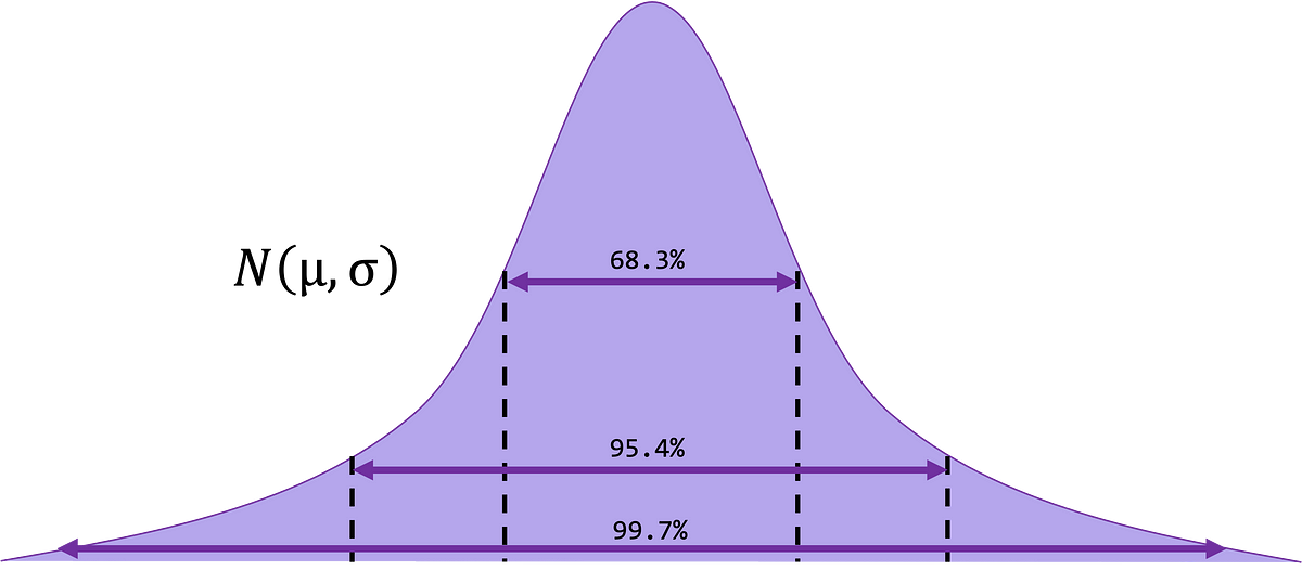
It’s unlikely that any explicit pattern imply will probably be precisely equal to the inhabitants imply, μ. Why, you make ask? Attributable to sampling error. To permit for sampling error, a parameter is often estimated to be inside a variety of values, referred to as a confidence interval. These intervals give a set of believable values for the true parameter.
Extra formally, a confidence interval is the likelihood that the interval will include the true worth (inhabitants parameter or level estimate) if we repeatedly sampled the inhabitants and carried out the calculations. Mentioned one other manner, how shut is our grouping of the purpose estimates we acquire from our pattern? We derive a confidence interval through the use of knowledge obtained from a pattern and specifying the boldness degree we want to have in our estimate. Three frequent confidence intervals used are the ninetieth, ninety fifth and the 99th percentile.
The formulation for the boldness interval of the parameter (inhabitants) imply for a selected degree alpha (α), when σ is understood will be calculated by:

- α : significance degree
- α = 1 — confidence intervals
- 90% confidence interval: z_α/2 = 1.65
- 95% confidence interval: z_α/2 = 1.96
- 99% confidence interval: z_α/2 = 2.58
Confidence Intervals for One Inhabitants Imply When σ is Recognized
Given the boldness interval 1 – α, we have to discover the related z-score (crucial worth) from a z-score distribution desk. One other strategy to write the equation prior as as proven right here:

- Xbar : pattern imply
- z_α/2 : z-score/crucial worth
- σ : inhabitants normal deviation
- n : pattern dimension
Instance. If you happen to wished to make sure 95% of the time the inhabitants imply (parameter imply) would land inside a variety of values you specify, decide the boldness interval based mostly on the pattern imply, Xbar. A ninety fifth confidence interval interprets to α = 0.05. So let’s calculate this based mostly on the equation specified beforehand.


One Pattern z-Interval
Our goal is to discover a confidence interval for a inhabitants imply, μ. Our assumptions embrace that our pattern was random, that our pattern is generally distributed or giant sufficient that we are able to assume it’s (n ≥ 30), and that the usual deviation σ is understood. We’d like σ as a way to carry out the calculate as per the formulation above.
1. Determine a confidence degree (1 – α)
2. Utilizing a z-table, discover z_{α/2}
3. The boldness interval for inhabitants/parameter imply, μ ranges from

the place z_{α/2} is derived from step 1, n is the pattern dimension and xbar is the imply computed from the pattern knowledge.
4. Interpret your findings. This implies stating “Our inhabitants imply, μ will fall inside the vary (__,__), (confidence degree) quantity of the time.
Notice that the boldness interval is taken into account to be precise for regular populations and is roughly appropriate for giant samples from non-normal populations [1].
Instance. Right here we have now the costs of a can of cat meals from 32 completely different shops in downtown Chicago. Discover a 95% confidence interval for the imply value of cat meals, μ, of all of the pet shops in downtown Chicago. Assume that the inhabitants normal deviation of the ages is 0.8 {dollars}.
1.96 2.43 2.32 2.45 2.00 3.21 2.97 1.90 3.04 1.63 3.31 2.39 2.00 2.78 3.45 3.54 4.70 3.82 4.15 3.16 3.54 2.49 2.96 3.35 2.47 2.94 1.96 3.40 1.74 1.51 2.23 1.66
As a result of the inhabitants normal deviation is understood, pattern dimension is 32, which is giant (≥30), we are able to use the one pattern z-interval when σ is understood to seek out the required confidence interval.

The boldness interval for the true inhabitants imply goes from 2.32 to 2.88 {dollars}. Our interpretation of that is as follows: We will be 95% assured that the imply value of a can of cat meals in downtown Chicago is someplace between 2.32 and a pair of.88 {dollars}.
Accuracy
“Accuracy is true to intention, precision is true to itself” — Simon Winchester [2]
Accuracy is a loaded time period, however regardless it implies there’s a floor fact by which we as evaluators can assess how appropriate or shut we’re to that floor fact. To that finish, because the width of our confidence interval will increase, the accuracy of our estimate decreases. Intuitively this could make sense as a result of there are extra potential level estimates for the parameter now contained inside that vary. For instance, a 95% confidence interval (2.32, 2.88) versus a 99% confidence interval (2.24, 2.96) as per the instance above. As we are able to plainly see, the second is wider. That is mediated by the actual fact we have now to be MORE certain our estimate falls on this vary. Within the earlier instance Xbar is 2.6, so with a 95% confidence degree, the error in our estimation is 2.6–2.32 = 0.28 {dollars}, and on the 99th the error in our estimation is 2.6–2.24 = 0.36 {dollars}.

Half the vary of our confidence interval (latter portion of our equation) will be parsed out as present under. That is known as our margin of error, denoted by E. It represents the most important potential distinction in our parameter estimate and our parameter worth as based mostly on our confidence degree.

this equation, if we have now a pre-specified confidence degree (z_{α/2}) we’re working in the direction of, how can we lower the error E (i.e. improve the accuracy of our estimate)?
INCREASE THE SAMPLE SIZE!
Since ’n’ is the one variable within the denominator, it is going to be the one factor we are able to simply do to lower ‘E’, since we are able to’t power our inhabitants to have a unique normal deviation.
Pattern Dimension
Suppose we’d prefer to have a smaller margin of error. And say we should be certain 90% of the time the inhabitants imply can be coated inside 0.2 {dollars} of the pattern imply. What pattern dimension would we’d like to have the ability to state this (assume σ = 0.8)?
We are able to remedy for n within the margin of error formulation:

We should always all the time spherical up when figuring out pattern dimension ’n’ from a margin of error. That is so E is rarely bigger than we would like.
How can we use what we’ve realized about confidence intervals to reply questions similar to…
- Will a brand new medicine decrease an individual’s a1c (lab used to detect diabetes)?
- Will a newly designed seatbelt scale back the variety of driver casualties in automotive accidents?
A lot of these questions will be addressed by statistical speculation testing — a decision-making course of for evaluating claims a couple of inhabitants.
Speculation Testing (Intuitive)
Let’s say I complain that I solely earn $1,000 a 12 months, and also you imagine me. Then, I invite you to tag alongside, and we climb into my BMW, drive to my non-public hangar to get in my non-public jet, and fly to my 3,000 sq. ft. residence in downtown Paris. What’s the very first thing you concentrate on my grievance? That I’m a liar…
Speculation Testing (Logic)
- You assume a sure actuality (I earn $1,000 yearly)
- You observe one thing associated to the belief (you noticed all my belongings)
- You assume, “How possible is it that I might observe what I’ve noticed, based mostly on the belief?”
- If you don’t imagine it to be possible (i.e. little probability it could occur, as on this case), you reject the belief. If you happen to imagine it to be possible (i.e. sufficient probability of this taking place) you don’t reject it and preserve going.
Speculation Testing (Formal)
A statistical speculation is a postulation a couple of inhabitants parameter, sometimes μ. There are two elements to formalizing a speculation, a null and different speculation.
- Null speculation (H₀): A statistical speculation that states {that a} parameter is the same as a selected worth (or units of parameters in numerous populations are the identical).
- Different speculation (Ha or H₁): A statistical speculation that states {that a} parameter is both < (left-tailed), ≠ (two-tailed) or > (right-tailed) than a specified worth (or states that there’s a distinction amongst parameters).
So our steps to speculation take a look at go as follows:
- State our null and different hypotheses — H₀ and H₁
- Decide from our hypotheses if this consistutes a proper, left or two-tailed take a look at
- Verify our significance degree alpha.
- Primarily based on alpha, discover the related crucial values from the suitable distribution desk (these differ based mostly on the sorts of ‘tails’ you may have and will present the directionality on the high of the desk)
- Compute the take a look at statistic based mostly on our knowledge
- Evaluate our take a look at statistic to our crucial statical worth
- Make the choice to reject or not reject the null speculation. If it falls in rejection area, reject in any other case settle for the null
- Interpret your findings — ‘there’s enough proof to help the rjeection of the null’ OR ‘there’s not enough proof to reject the null speculation’
A take a look at statistic is a calculated worth based mostly on our collected from a pattern and is in contrast in opposition to the a-priori threshold (crucial worth) to find out significance. Important values act because the boundary separating the area of rejection and non-rejection (significance and non-significance). These are decided based mostly on the related statistic desk. We’ve got mentioned the z-table to this point however will cowl different statistical tables in subsequent bootcamps. See the determine under for a visible illustration of how a two-tailed (two rejection areas).

Reject Areas
A part of our speculation testing is deciding which manner we anticipate the connection to be, and thus which ‘tail’ we will probably be investigating. There are 3 choices obtainable — two-tailed, left-tailed and right-tailed. In a two-tailed take a look at, the null speculation is rejected when the take a look at statistic is both smaller OR bigger (rejections areas on left AND proper sides) than our crucial statistic worth (decided a-priori). That is synonymous with investigating ‘is that this completely different than the crucial worth no matter route?’. In a left-tailed take a look at, the null speculation is rejected solely when the take a look at statistic is smaller (rejection space is on the left) than the crucial statistic. Lastly, in a right-tailed take a look at, the null speculation is rejected when the take a look at statistic is bigger (rejection space is on the best facet of the bell curve) than the crucial statistic. See the determine under:

Conclusion from Speculation Checks
If a speculation take a look at is performed to reject the null speculation (H₀), we are able to make the conclusion that: “based mostly on our pattern, the take a look at result’s statistically vital and there’s enough proof to help the choice speculation (H₁) which may now be handled as true”. In actuality, we hardly ever know the inhabitants parameter. Thus, if we don’t reject the null speculation, we have to be cautious and non overstate our findings by concluding that the information didn’t present enough proof to help the choice speculation. For instance, ‘There may be not enough proof/info to find out that the null speculation is fake.’
One-Pattern z-Check
In a one-sample z-test, we’re evaluating a single pattern to info from the inhabitants through which it arises. It is likely one of the most simple statistical checks we are able to take a look at our speculation by following these 8 steps:
1. The null speculation is H0: μ = μ₀, and the choice speculation is considered one of 3 potential choices relying on whether or not route issues, and in that case which manner:

2. Decide the directionality of the take a look at — which tail(s) you’re investigating

3. Determine on a significance degree, α.
4. Primarily based on alpha, discover the related crucial values from the suitable distribution desk (these differ based mostly on the sorts of ‘tails’ you may have and will present the directionality on the high of the desk)
5. Compute the take a look at statistic based mostly on our knowledge

6. Evaluate our take a look at statistic to our crucial statical worth — is Zcalc >,<, ≠ ?

7. Make the choice to reject or not reject the null speculation. If it falls in rejection area, reject in any other case settle for the null
8. Interpret the findings— ‘there’s enough proof to help the rejection of the null’ OR ‘there’s not enough proof to reject the null speculation’
Instance. A physician is interested by discovering out whether or not a brand new bronchial asthma medicine may have any undesirable unwanted side effects. Particularly, the physician is worried with the spO2 of their sufferers. Will the spO2 stay unchanged after the medicine is run to the affected person? The physician is aware of the typical spO2 for an in any other case wholesome inhabitants is 95%, the hypotheses for this case are:

That is referred to as a two-tailed take a look at (if H₀ is rejected, μ will not be equal to 95, thus it may be both lower than or larger than 95). We’ll take a look at find out how to comply with this up in a following bootcamp. What if the query was whether or not the spO2 decreases after the medicine is run?

That is notation for a left-tailed take a look at (if H0 is rejected, μ is taken into account to be lower than 95). What if the query was whether or not the spO2 will increase after the medicine is run?

That is the notation for a right-tailed take a look at (if H0 is rejected, μ is taken into account to be larger than 95).
Instance. A local weather researcher needs to see if the imply variety of days of >80 levels Fahrenheit within the state of California is larger than 81. A pattern of 30 cities in California are chosen randomly has a imply of 83 days. At α = 0.05, take a look at the declare that the imply variety of days of >80 levels F is larger than 81 days. The usual deviation of the imply is 7 days.
Let’s examine our assumptions: 1) we have now obtained a random pattern, 2) pattern dimension is n=30, which is ≥ 30, 3) the usual deviation of the parameter is understood.
- State the hypotheses. H0: μ = 81, H1: μ ≥ 81
- Set a significance degree, α = 0.05
- Directionality of the take a look at: right-tailed take a look at (since we’re testing ‘larger than’)
- Utilizing α = 0.05 and understanding the take a look at is right-tailed, the crucial worth is Zcrit = 1.65. Reject H0 if Zcalc > 1.65.
- Compute the take a look at statistic worth.

6. Evaluate the Zcalc and Zcrit. Since Zcalc = 1.56 < Zcrit = 1.65,
7. Zcalc doesn’t fall into the reject area, subsequently, we fail to reject the null speculation.

8. Interpret our findings. There may be not sufficient proof to help the declare that the imply variety of days is larger than 81 days.
Instance. The residence affiliation of Chicago stories that the typical price of hire for a 1 bed room residence downtown is $2,200. To see if the typical price at a person residence constructing is completely different, a renter selects a random pattern of 35 residences inside the constructing and finds that common price of a 1-BR residence is $1,800. The usual deviation (σ) is $300. At α = 0.01, can or not it’s concluded that the typical price of a 1-BR at a person residence is completely different from $2,200?
Let’s examine our assumptions: 1) we have now obtained a random pattern, 2) pattern is 35, which is ≥ 30, 3) the usual deviation of the inhabitants is supplied.
- State the hypotheses. H0: μ = 2,300, H1: μ ≠ 2,200
- α = 0.01
- Directionality of the take a look at: two-tailed
4. Discover the crucial worth, based mostly on the z-table. Since α = 0.01 and the take a look at is a two-tailed take a look at, the crucial worth is Zcrit(0.005) = ±2.58. Reject H0 if Zcalc > 2.58 or Zcalc < -2.58.
5. Compute the z-test statistic

6. Evaluate the calculated statistic in opposition to the one decided from step 2
7. Since Zcalc = -7.88 < -2.58, it falls into the rejection area, we reject H0.
8. Interpret our findings. There may be enough proof to help the declare that the typical price of a 1-BR residence at that particular person residence constructing is completely different from $2,200. Particularly, it’s CHEAPER than the parameter imply.
We’ve coated find out how to acquire confidence in our statistical estimates generated from our knowledge by the usage of confidence intervals. After studying this text you must have a agency grasp of the which means of small versus giant confidence intervals and the implications from an inference standpoint. Within the engineering world we talk about tolerances on machined elements and mathematical ‘tolerances’ aren’t any exception. Right here we often quantify our mathematical estimates utilizing the time period repeatability. We are able to outline repeatability as the flexibility to generate the identical consequence constantly. If a metric or design doesn’t have repeatability, it could produce scattered outcomes (i.e. wider confidence intervals).
The subsequent bootcamp will entail detailing the trade-off between sort 1 and a pair of errors, so keep tuned!
Earlier boot camps within the collection:
#1 Laying the Foundations
#2 Middle, Variation and Place
#3 Most likely… Likelihood
#4 Bayes, Fish, Goats and Automobiles
#5 What’s Regular
All photos except in any other case said are created by the creator.
References
[1] Allan Bluman, Statistics, E. Elementary Statistics.
[2] Winchester, Simon. The perfectionists: how precision engineers created the trendy world. HarperLuxe, 2018.
