Be taught the mathematics and strategies behind the libraries you employ day by day as an information scientist

To extra formally handle the necessity for a statistics lecture collection on Medium, I’ve began to create a collection of statistics boot camps, as seen within the title above. These will construct on each other and as such shall be numbered accordingly. The motivation for doing so is to democratize the data of statistics in a floor up vogue to deal with the necessity for extra formal statistics coaching within the knowledge science neighborhood. These will start easy and increase upwards and outwards, with workout routines and labored examples alongside the best way. My private philosophy relating to engineering, coding, and statistics is that for those who perceive the mathematics and the strategies, the abstraction now seen utilizing a large number of libraries falls away and permits you to be a producer, not solely a shopper of knowledge. Many sides of those shall be a overview for some learners/readers, nevertheless having a complete understanding and a useful resource to discuss with is vital. Completely happy studying/studying!
This bootcamp is devoted to introducing Bayes theorem and doing a deeper dive into some chance distributions.
Bayes’ rule is the rule to compute conditional chance. Some background on Bayes:
- Used to revise possibilities in accordance with newly acquired data
- Derived from the final multiplication rule
- ‘As a result of this has occurred’… ‘This is kind of probably now’ and many others.
Supposed that occasions A1, A2, …Ak are mutually unique and exhaustive (as coated in our earlier bootcamp). Then for any occasion B:
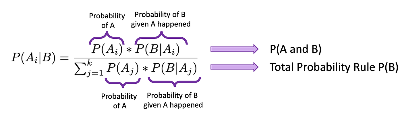
P(A) is the chance of occasion A when there isn’t a different proof current, referred to as the prior chance of occasion A (base price of A). P(B) is the whole chance of taking place of occasion B, and might be subdivided into the denominator within the equation above. P(B) is known as the chance of proof, and derived from the Whole Chance Rule. P(B|A) is the chance of taking place an occasion B provided that A has occurred, generally known as the probability. P(A|B) is the chance of how probably A occurs provided that B has already occurred. It is called posterior chance. We are attempting to calculate the posterior chance.
What if (from bootcamp 3) in examples of low, medium, and high-risk for stroke and the chance of getting a stroke in 5 years, the query was “If a randomly chosen topic aged 50 had a stroke previously 5 years, what’s the chance that he/she was within the low-risk group?” Moreover, you’re given the identical possibilities as beforehand (seen beneath).
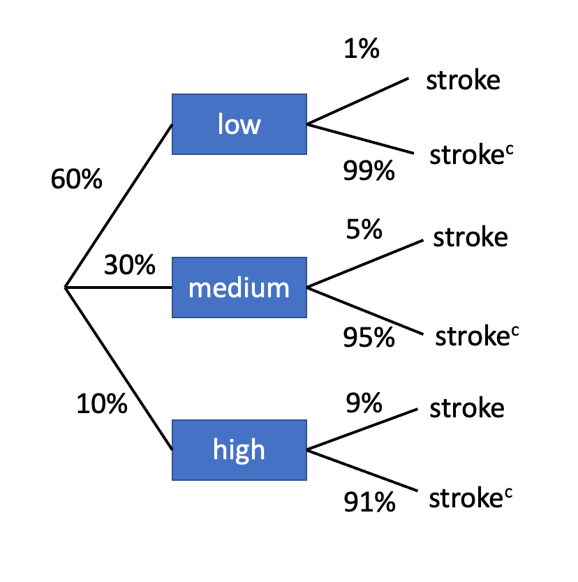
P(low) = 0.6, P(medium) = 0.3, P(excessive) = 0.1
P(stroke|low) = 0.01, P(stroke|medium) = 0.05, P(stroke|excessive) = 0.09
P(low|stroke) = ? (that is our posterior chance)

So our reply is that if a randomly chosen topic aged 50 had a stroke previously 5 years, what’s the chance that he/she was within the low-risk group is 20%.
Let’s consider the traditional Monty corridor downside. Behind two of those doorways, there’s a goat, behind the third is your dream automobile. You choose a door. One of many different doorways is opened to disclose a goat, not your present choice. Monty asks for those who want to keep together with your door or swap to the opposite door. What must you do? You must swap — however WHY?! Let’s have a look…
While you chosen the door the primary time you have got a 1/3 or 33.33% of choosing accurately (by random) — that is going to alter. Let’s say the automobile is behind door 1 and also you picked door 2 …so you’re presently in possession of a goat. Monty KNOWS the place the automobile is. He CANNOT open your door OR the place the automobile is. So must you keep or swap? You may have simply been given 33.33% extra so it’s best to swap!
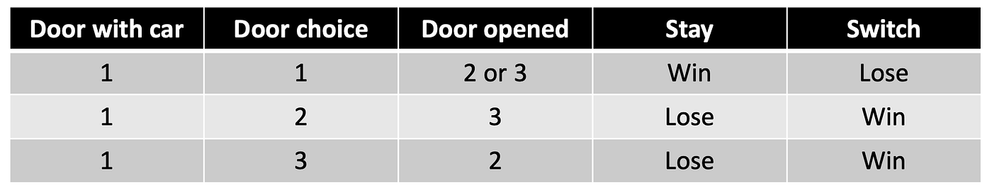
Because of this it’s a conditional chance downside. Now we have conditioned on the ‘door opened’ the second time you could decide. If we play this out over all situations and all door picks, the identical chance holds. If Monty opened a door RANDOMLY your possibilities of profitable the automobile can be 50% the second time not 66.6% for switching and 33.33% for staying.
Random Variables
A random variable is a quantitative variable whose worth will depend on probability. Examine this with a discrete random variable, which is a random variable whose potential values might be listed.
Instance. Every single day, Jack and Mike keep the most recent within the biology lab and toss a coin to determine who will clear up the lab. If it’s heads (H), then Jack will clear up. If it’s tails (T), Mike will do the work. For 3 consecutive days, they report back to their lab supervisor. The pattern area is:
{H,H,H} {H,H,T} {H,T,T} {T,H,T} {H,T,H} {T,H,H} {T,T,H} {T,T,T}
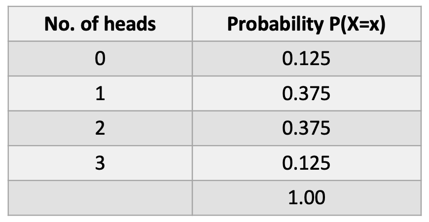
What’s the chance that Jack cleans up the lab 0, 1, 2, or 3 occasions? (let ‘x’ be the variety of occasions Jack cleans).
Right here is the theoretical or anticipated chance distribution:
Now carry out 1000 observations of the random variable X (the variety of heads obtained in 3 tosses of a balanced coin). That is the empirical chance distribution (noticed).
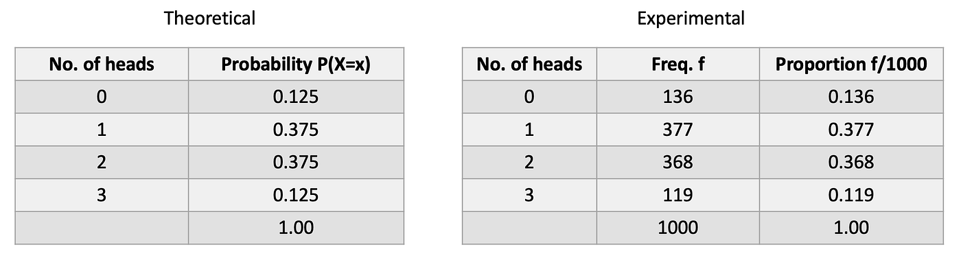
Notice that the possibilities within the empirical distribution are pretty near the possibilities within the theoretical (true) distribution when the variety of trials are massive.
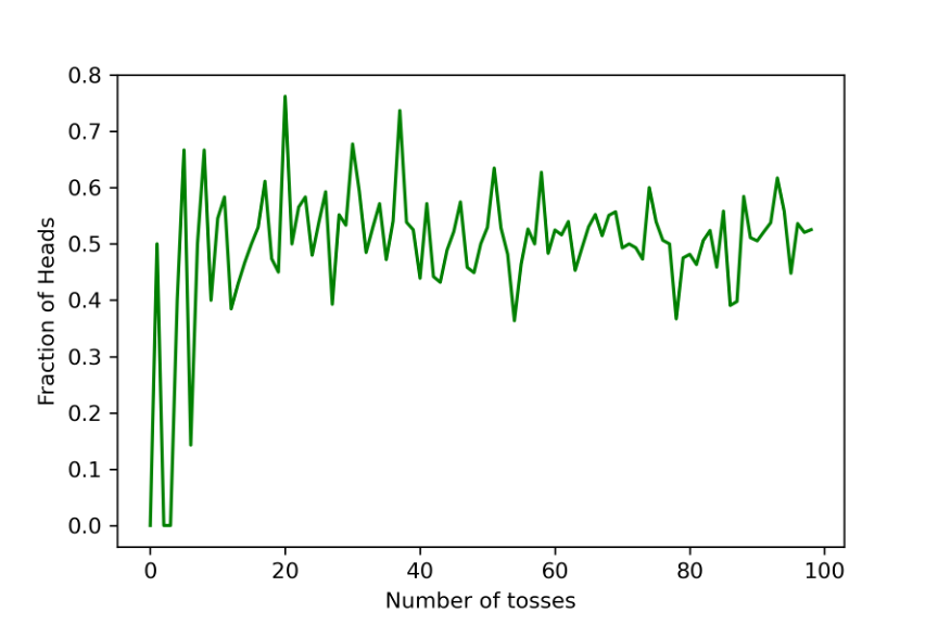
Legislation of Giant Numbers
If we tossed a balanced coin as soon as, we theorize that there’s 50–50 probability the coin will land with heads going through up. What occurs if the coin is tossed 50 occasions? Will head come up precisely 25 occasions? Not essentially, resulting from variation. The legislation of huge numbers states that because the variety of trials will increase, the empirical chance (estimated chance from observations) will method the theoretical chance. On this case, 1/2. You possibly can see within the graph beneath the fraction of heads approaches the theoretical the extra tosses are carried out.
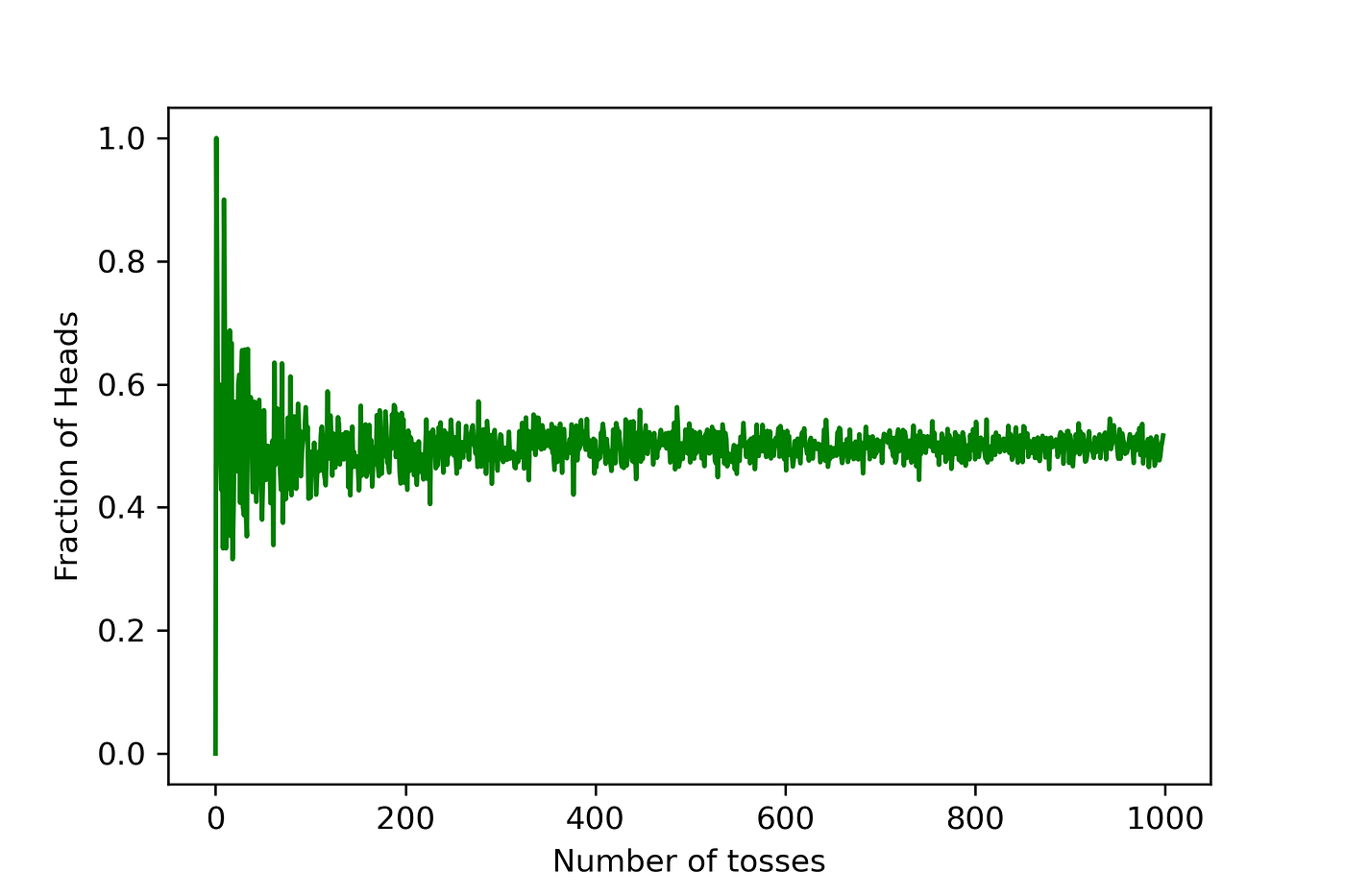
Right here is the code to generate the above determine in python:
from random import randint
import matplotlib.pyplot as plt
import numpy as np
import pandas as pd
#num = enter('Variety of occasions to flip coin: ')
fracti = []
tosses = []
for num_tosses in vary(1,1000):
flips = [randint(0,1) for r in range(int(num_tosses))]
outcomes = []
for object in flips:
if object == 0:
outcomes.append(1)
elif object == 1:
outcomes.append(0)
fracti.append(sum(outcomes)/int(num_tosses))
tosses.append(flips)df = pd.DataFrame(fracti, columns=['toss'])
plt.plot(df['toss'], colour='g')
plt.xlabel('Variety of tosses')
plt.ylabel('Fraction of Heads')
plt.savefig('toss.png',dpi=300)
Necessities of a chance distribution:
- The sum of the possibilities of a discrete random variable should equal 1, ΣP(X=x)=1.
- The chance of every occasion within the pattern area should be between 0 and 1 (inclusive). I.e. 0≤ P(X) ≤1.
The chance distribution is similar because the relative frequency distribution, nevertheless, the relative frequency distribution is empirical and the chance distribution is theoretical.
Discrete Chance Distribution Imply or Expectation
The imply of a discrete random variable X, is denoted μ_x or, when no confusion will come up, merely, μ. it’s outlined by:
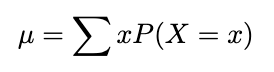
The phrases anticipated worth and expectation are generally used instead of the time period imply — and why if you see the capital ‘𝔼’ for expectation, it’s best to assume ‘imply’.
To interpret the imply of a random variable, think about numerous impartial observations of a random variable X. The common worth of these commentary will roughly equal the imply, μ, of X. The bigger the variety of observations, the nearer the common tends to be to μ.
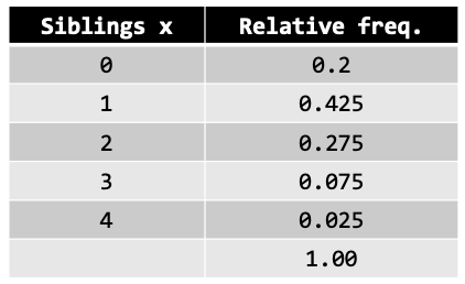
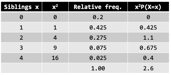
The relative frequency desk truly is a discrete chance distribution, which comprises random variable (siblings x) and chance of every occasion (relative frequency). Given the siblings chance distribution within the class, discover the anticipated quantity (imply) of siblings on this class. The desk beneath footwear the relative frequency distribution.
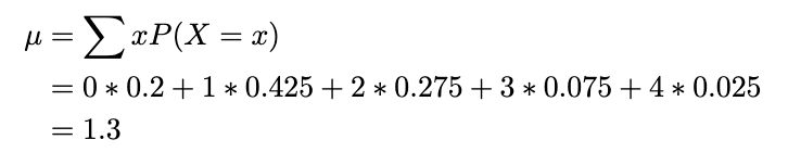
Calculating the imply:
Discrete Chance Distribution Customary Deviations
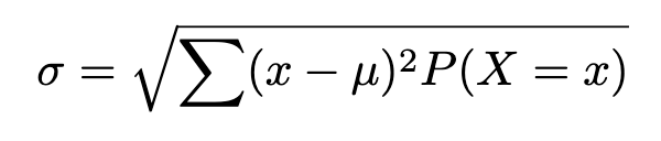
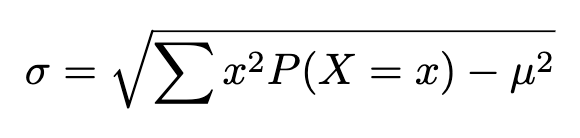
The usual deviation of a discrete random variable X, is denote σ_x, or, when no confusion will come up, merely, σ. It’s outlined as:
The usual deviation of a discrete random variable will also be obtained from the computing components:
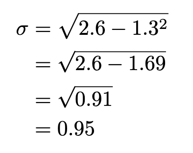
Performing the working on our identical frequency distribution:
Discrete Chance Distribution Cumulative Chance
Instance. Flip a good coin 10 occasions. What’s the chance of getting at most 3 heads?
lets X = complete variety of heads
P(X≤3)= P(X=0)+P(X=1)+P(X=2)+P(X=3)
What’s the chance of getting at least 3 heads?
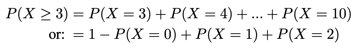
P(X≥3)= P(X=3)+P(X=4)+P(X=5)+..+P(X=10)
=1- P(X=0)+P(X=1)+P(X=2)
=1-P(X≤2)
What’s the chance of getting between 2 and 4 (inclusive)?
P(2≤X≤4)= P(X≤4)-P(X<2)
= P(X≤4)-P(X≤1)
= P(X=4)+P(X=3)+P(X=2)
A Bernoulli trial represents an experiment with solely 2 potential outcomes (e.g. A and B). The components is denoted as:
P(X=A) = p, P(X=B) = 1-p=q
p : chance of on the outcomes (e.g. A)
1-p : chance of the opposite final result (e.g. B)
Examples:
- flipping a coin
- passing or failing an examination
- task of remedy/management group for every topic
- check constructive/unfavorable in a screening/diagnostic check
A binomial experiment is the concatenation of a number of Bernoulli trials. It’s a chance experiment that should fulfill the next necessities:
- Should have a set variety of trials
- Every trial can solely have 2 outcomes (e.g. success/failure)
- Trials MUST be impartial
- Chance of success should stay the identical for every trial
A binomial distribution is a discrete chance distribution of the variety of successes in a collection of ’n’ impartial trials, every having two potential outcomes and a continuing chance of success. A Bernoulli distribution might be thought to be a particular Binomial distribution when n=1.
Notation:
X~Bin(n,p)
p: chance of success (1-p: chance of failure)
n: variety of trails
X: variety of success in n trials, with 0≤X≤n
Making use of counting guidelines:
‘X’ successes in ‘n’ trials → p*p*…*p= p^X
n-X: failure → (1-p)*(1-p)*…*(1-p)= (1-p)^(n-X) = q^(n-X)
Binomial Chance System (theoretical):
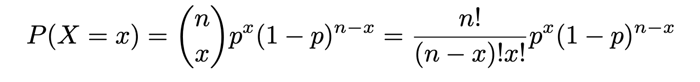
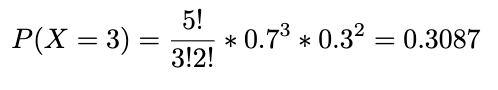
Instance. Every single day, Adrienne and Banafshe keep the most recent within the engineering lab and toss a coin to determine who will clear up the lab. If it’s heads (H), Adrienne will do the work, if tails (T), Banafshe. The coin they used, nevertheless, has a 0.7 chance of getting heads. Within the following week, discover the chance that Adrienne will clear up the lab or precisely 3 days (per week right here is the 5 day work week). Let X denote the variety of days in per week Adrienne cleans up the lab. X~Bin(5,0.7).
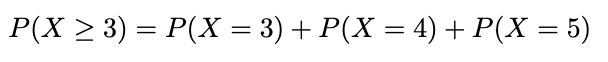
What’s the chance that Adrienne will clear up for a minimum of 3 days? We will categorical it beneath and undergo the identical calculation as above including the possibilities for X=3, X=4, and X=5.
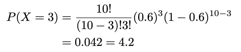
Instance. A publication entitled Statistical report on the well being of People indicated that 3 out of 5 People aged 12 years and over visited a doctor a minimum of as soon as previously 12 months. If 10 People aged 12+ years are randomly chosen, discover the chance that precisely 3 individuals visited a doctor a minimum of as soon as final 12 months. Discover the chance that a minimum of 3 individuals visited a doctor a minimum of yearly.
n: variety of trials=10
X: Variety of successed (visited a doctor) in n trials = 3
p: numerical chance of success = 3/5
q: numerical chance of failure = 2/5
and:
Imply and Stand. Dev of Binomial Distributions
- imply: μ=n*p
- variance: σ² = n*p*q
- customary deviation: σ= sqrt(n*p*q)
Instance. What’s the imply and customary deviation of the variety of cleansing up Adrienne will do in per week?
n=5, p=0.7, q=0.3
μ = 5*0.7 = 3.5
σ = sqrt(5*0.7*0.3) = 1.02
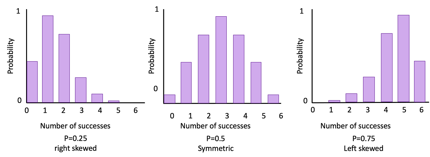
Typically, a binomial distribution is true skewed if p<0.5, is symmetric if p=0.5, and left skewed if p>0.5. The determine beneath illustrates these information for 3 totally different binomial distributions with n=6.
Greater than 2 outcomes?
What if we’ve greater than two outcomes? Say we’re wanting on the M&M’s Cynthia had. We decide 5 with our eyes closed from the field. What’s the probability we could have 2 blue, 1 yellow, 1 purple and 1 inexperienced?
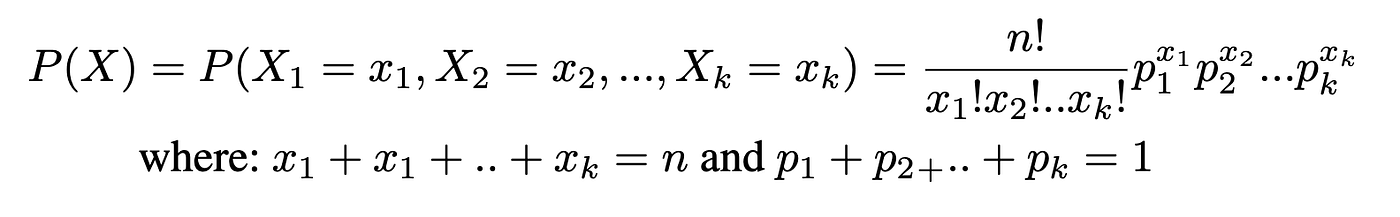
A multinomial distribution is a distribution during which every trial has greater than 2 impartial outcomes. If X consists of conserving monitor of ok mutually unique and exhaustive occasions E1, E2,..Ek what have corresponding possibilities p1, p2,..pk of occurring, and the place X1 is the variety of occasions E1 will happen, X2 is the variety of occasions E2 will happen, and many others., then the chance that X (a selected taking place of x1, x2, ..) will happen is:
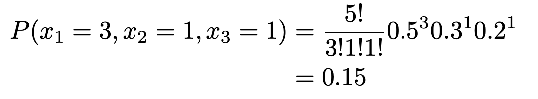
Instance. In a big metropolis, 50% of the individuals select a film, 30% select dinner and a play, and 20% select buying, as probably the most favorable leisure exercise. If a pattern of 5 persons are randomly chosen, discover the chance that 3 are planning to attend a film, 1 to a play, and 1 to a shopping center.
n=5, x1=3, x2=1, x3=1, p1=0.5, p2=0.3, p3=0.2
Now, say we wish to plan for avoiding overcrowding within the ER. If we all know there are 25,000 visits a 12 months (three hundred and sixty five days) at Northwestern Medication, and the ER handles 60 effectively a day, what’s the probability we’ll get 68 a day?
Say a bakery is not going to cost their muffins in the event that they don’t have sufficient chocolate chips, how may we mannequin this?
The proper pronunciation of Poisson is pwa-sawn, and it means fish in French! A Poisson distribution is a kind of discrete chance distribution, that fashions the frequency with which a specified occasion happens throughout a selected time period, quantity, are and many others. (e.g. variety of chocolate chips per muffin  ). Formally, it’s the chance of X occurrences in an interval (quantity, time and many others.) for a variable the place λ is the imply variety of occurrences per unit (time, quantity and many others.)
The components is:
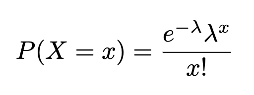
x=0,1,2,…(# of occurrences), e=is the exponential operate
- imply: μ = λ
- variance: σ² = λ
- customary deviation: sqrt(λ)
Discover that the imply and the variance are the sam within the Poisson distribution!
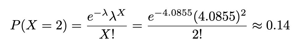
Instance. Within the black hawks season, 203 accidents had been discovered over 49,687 sport hours. Discover the chance that 2 accidents occurred inside 1000 sport hours.
1. Discover the harm price per 1000 sport hours
2. X = 2, the place X ~ Poisson (λ=4.0855):
Meals for thought, actually. Suppose the identical bakery as earlier than, has low-cost stale croissants and contemporary croissants, the beginner on the bakery combined all of them up. There have been 14 contemporary and 5 stale. If you wish to buy 6 croissants, what are the possibilities of getting just one stale?
A hypergeometric distribution is a distribution of a variable that had two mutually unique outcomes when sampling is completed WITHOUT alternative. It’s often used when inhabitants dimension is small.
Given a inhabitants of two sorts of objects, such that there are ‘a’ gadgets of sort A and ‘b’ gadgets of sort B and a+b equals the whole inhabitants, and we wish to select ’n’ gadgets. What’s the chance of choosing ‘x’ variety of sort A gadgets?
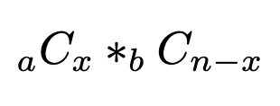
Step 1. The variety of methods to pick out x gadgets of sort A (x gadgets from sort A, so the remainder n-x gadgets should be from sort B):
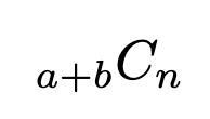
Step 2. The overall variety of methods to pick out n gadgets from the pool of (a+b):
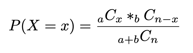
So the chance P(X=x) if choosing, with out alternative in a pattern dimension of n, X gadgets of sort A and n-X gadgets of sort B:
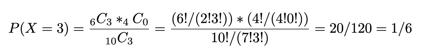
Instance. 10 individuals apply for a place of analysis coordinator for a basketball research. Six have accomplished a postgraduate diploma and 4 haven’t. If the investigator of the research selects 3 candidates randomly with out alternative, discover the chance that each one 3 had postgraduate levels.
a=6 having postgrad levels
b=4 no postgrad levels
n=3
X=3
On this bootcamp, we’ve continued within the vein of chance principle now together with work to introduce Bayes theorem and the way we are able to derive it utilizing our beforehand realized guidelines of chance (multiplication principle). You may have additionally realized how to consider chance distributions — Poisson, Bernoulli, Multinomial and Hypergeometric. Look out for the following installment of this collection, the place we’ll proceed to construct our data of stats!!
Earlier boot camps within the collection:
#1 Laying the Foundations
#2 Middle, Variation and Place
#3 Chance… Chance
All pictures until in any other case acknowledged are created by the creator.
