
The very best benchmarked mannequin within the M4 competitors simply skilled, tuned, and examined utilizing Python

Lesser recognized than a classical approach like ARIMA, Theta is a time collection mannequin that produces correct outcomes and is straightforward to know and apply. It’s a good instrument to have within the arsenal if you’re a time collection practitioner and forecaster.
It really works by extracting two “theta traces” from an underlying time collection. The primary line is the time collection’ linear development and will be extracted by operating a easy linear regression on the information that makes use of a time development because the enter. This theta line will be extrapolated to the long run fairly just by persevering with its linear development indefinitely.
The second theta line will be considered the collection’ curvature. It’s the collection’ second distinction multiplied by an element, by default, 2. Values lower than 1 dampen the curvature and emphasize long-term traits and larger than 1 intensify it and emphasize short-term traits. This second theta line is extrapolated ahead through the use of exponential smoothing.
These two theta traces are then mixed in both an additive or multiplicative course of. To account for seasonality, the mannequin additionally de-seasons the information with both a multiplicative or additive seasonal decomposition technique earlier than extracting the theta traces. This seasonality is then re-applied to the information within the forecast after the theta traces are mixed.
The paper that proposes this technique additionally mentions that additional analysis may embody extracting greater than two theta traces, however so far as I’m conscious, no such fashions have turned up something promising, however it’s attention-grabbing to consider (Assimakopoulos & Nikolopoulos, 2000).
Quite simple, proper? Let’s take a look at the way to use Python to implement it.
Darts
Darts is a user-friendly time-series package deal that makes use of an implementation of the theta mannequin which known as FourTheta, a spinoff of the concept defined above that may apply exponential transformations to the primary theta line (as a substitute of utilizing a easy linear development). This spinoff of the mannequin was the top-performing benchmark mannequin within the M4 competitors held in 2020.
To put in darts:
pip set up darts
Here’s a hyperlink to the mannequin documentation in darts.
Scalecast
Scalecast ports the theta mannequin from darts into a standard time-series framework that’s easy-to-implement and evaluate towards a number of different classical time collection approaches, machine studying fashions from scikit-learn, and different strategies. I will likely be demonstrating the scalecast implementation of the theta mannequin as a result of I’m the creator of scalecast and need to present how this framework will be applied very simply for any consumer. That being mentioned, if you wish to use the mannequin from darts immediately, it’s also provides a user-friendly and cozy framework.
To put in scalecast:
pip set up scalecast
You could find the entire pocket book used on this article right here. The info is open-access from the M4 competitors and is on the market on GitHub. We will likely be utilizing the H7 hourly time collection.
Code Implementation
Making use of this mannequin in code could be very easy. We first load our information to a Forecaster object:
prepare = pd.read_csv('Hourly-train.csv',index_col=0)
y = prepare.loc['H7'].to_list()
current_dates = pd.date_range(
begin='2015-01-07 12:00',
freq='H',
durations=len(y)
).to_list()
f = Forecaster(y=y,current_dates=current_dates)
We are able to plot this collection to have a greater thought what we’re working with:
f.plot()
plt.present()

Let’s put aside 25% of this information for testing and likewise forecast out 48 durations into the long run:
f.set_test_length(.25)
f.generate_future_dates(48)
Now, we will specify a hyperparameter grid to search out one of the best ways to tune this mannequin. This grid will work to discover a fairly good mannequin in most circumstances, however you can additionally take a look at including extra theta values to it.
from darts.utils.utils import (
SeasonalityMode,
TrendMode,
ModelMode
)theta_grid = {
'theta':[0.5,1,1.5,2,2.5,3],
'model_mode':[
ModelMode.ADDITIVE,
ModelMode.MULTIPLICATIVE
],
'season_mode':[
SeasonalityMode.MULTIPLICATIVE,
SeasonalityMode.ADDITIVE
],
'trend_mode':[
TrendMode.EXPONENTIAL,
TrendMode.LINEAR
],
}
Now, let’s use 3-fold time collection cross validation to search out the most effective hyperparameter mixture. This can create 3 segments of the information primarily based on our coaching set solely the place every validation set is 131 observations lengthy and fashions with all the above hyperparameter mixtures are skilled on the information that got here earlier than every validation set. The ultimate mannequin is chosen primarily based on which mannequin returned the most effective common MAPE worth throughout all folds.
f.set_validation_metric('mape')
f.set_estimator('theta')
f.ingest_grid(theta_grid)
f.cross_validate(ok=3)
The very best parameters chosen from cross validation had been:
>>> f.best_params
{'theta': 1,
'model_mode': <ModelMode.ADDITIVE: 'additive'>,
'season_mode': <SeasonalityMode.MULTIPLICATIVE: 'multiplicative'>,
'trend_mode': <TrendMode.EXPONENTIAL: 'exponential'>}
We then use that chosen mannequin to forecast into our check set and into our 48-period forecast horizon:
f.auto_forecast()
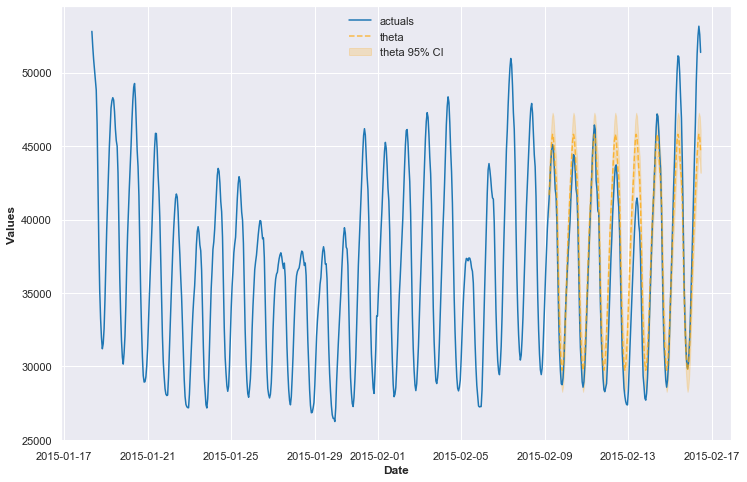
We are able to now see our check outcomes visualized:
f.plot_test_set(ci=True)
plt.present()
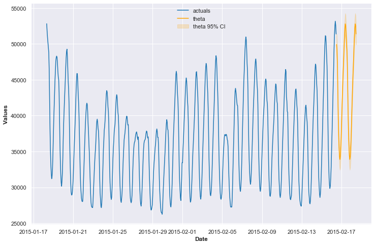
And the forecast outcomes:
f.plot(ci=True)
plt.present()
This returned a Take a look at-set MAPE results of 5.5%. The typical validation MAPE within the cross-validation course of was 7.5%. It is sensible that the validation MAPE could be barely worse because it had smaller coaching units to study from in every validation iteration.
Let’s say a while has passed by and we now have some new information to introduce to this mannequin and we will measure its efficiency over the 48-period forecast. Let’s see the way it did.
check = pd.read_csv('Hourly-test.csv',index_col=0)
y_test = check.loc['H7'].to_list()
future_dates = pd.date_range(
begin=max(current_dates) + pd.Timedelta(hours=1),
freq='H',
durations=len(y_test),
).to_list()fcst = f.export('lvl_fcsts')
mape = np.imply([(f - a) / a for f, a in zip(fcst['theta'],y_test)])
This returns a price of 6%, proper in between our test-set and validation metrics, precisely what we should always count on!
The theta mannequin is a robust instrument for time-series analysts that’s easy in idea, easy-to-tune, and straightforward to judge. I hope you discovered this tutorial helpful! In that case, please think about using scalecast sooner or later and contribute to its progress!
V. Assimakopoulos, Ok. Nikolopoulos, The theta mannequin: a decomposition method to forecasting, Worldwide Journal of Forecasting, Quantity 16, Concern 4, 2000, Pages 521–530, ISSN 0169–2070, https://doi.org/10.1016/S0169-2070(00)00066-2.
(https://www.sciencedirect.com/science/article/pii/S0169207000000662)
