
Shapiro-Wilk check, Kolmogorov–Smirnov check, and D’Agostino-Pearson’s K² check

Regular distribution, also called the Gaussian distribution, is a likelihood distribution described with two parameters: the imply and the usual deviation. For a standard distribution, 68% of the observations are inside ± one normal deviation of the imply, 95% are inside ± two normal deviations, and 99.7% are inside ± three normal deviations.
For most of the hottest statistical assessments, testing the normality is important to satisfy the assumptions. In any other case, we’d draw inaccurate conclusions and develop incorrect fashions.
However, to conclude the distribution of the information, statisticians mustn’t rely solely on graphical strategies equivalent to histograms or distribution plots. It’s also needed to incorporate the outcomes from the normality assessments.
Nonetheless, there are a number of assessments within the literature that can be utilized to evaluate this normality, turning into troublesome to find out which is probably the most correct one for our situation. For instance, the article [1] mentions 27 completely different normality assessments.
Therefore, the intention of this text is to explain and evaluate the three essential normality assessments:
- Shapiro-Wilk check
- Kolmogorov–Smirnov check
- D’Agostino-Pearson’s K² check
This text unfolds as follows. Firstly, an outline of every of these assessments (c.f., Part 1). Secondly, a comparability between the assessments and a conclusion about which is the optimum methodology to make use of (c.f., Part 2). Lastly, the implementation of these algorithms in Python (c.f., Part 3).
The speculation for the Shapiro-Wilk and D’Agostino-Pearson’s K² assessments are:
In distinction, the hypotheses for the Kolmogorov–Smirnov check are:
If we take into account that the desired distribution is the conventional distribution, then we’d be assessing the normality.
If the p-value is lower than the chosen alpha degree, then the null speculation is rejected and there may be proof that the information examined aren’t usually distributed. Alternatively, if the p-value is larger than the chosen alpha degree, then the null speculation can’t be rejected.
Here’s a step-by-step methodology to calculate the p-value for every of the assessments.
Shapiro-Wilk check
The fundamental strategy used within the Shapiro-Wilk (SW) check for normality is as follows [2].
Firstly, organize the information in ascending order in order that x_1 ≤ … ≤ x_n. Secondly, calculate the sum of squares as follows:

Then, calculate b as follows:

taking the ai weights from Desk 1 (based mostly on the worth of n) within the Shapiro-Wilk Tables. Observe that if n is odd, the median knowledge worth is just not used within the calculation of b. If n is even, let m = n/2, whereas if n is odd let m = (n–1)/2.
Lastly, calculate the check statistic:

Discover the worth in Desk 2 of the Shapiro-Wilk Tables (for a given worth of n) that’s closest to W, interpolating if needed. That is the p-value for the check.
This strategy is proscribed to samples between 3 and 50 parts.
Kolmogorov–Smirnov check
The Kolmogorov-Smirnov check compares your knowledge with a specified distribution and outputs if they’ve the identical distribution. Though the check is nonparametric — it doesn’t assume any specific underlying distribution — it’s generally used as a check for normality to see in case your knowledge is generally distributed [3].
The final steps to run the check are:
- Create an EDF on your pattern knowledge (see Empirical Distribution Operate for steps). The empirical distribution operate is an estimate of the cumulative distribution operate that generated the factors within the pattern.
- Specify a mother or father distribution (i.e. one that you just wish to evaluate your EDF to)
- Graph the 2 distributions collectively.
- Measure the best vertical distance between the 2 graphs and calculate the check statistic the place m and n are the pattern sizes.


- Discover the important worth within the KS desk.
- Examine to the important worth.
D’Agostino-Pearson’s K² check
The D’Agostino-Pearson’s K² check calculates two statistical parameters, named kurtosis and skewness, to find out if the information distribution departs from the conventional distribution:
- Skew is a quantification of how a lot distribution is pushed left or proper, a measure of asymmetry within the distribution.
- Kurtosis quantifies how a lot of the distribution is within the tail. It’s a easy and generally used statistical check for normality.
This check first computes the skewness and kurtosis to quantify how far the distribution is from Gaussian by way of asymmetry and form. It then calculates how far every of those values differs from the worth anticipated with a Gaussian distribution, and computes a single p-value from the sum of those discrepancies [4].
To reply this query, right here is the conclusion from the article Asghar Ghasemi et al. (2012) [5], which has over 4000 citations:
In response to the out there literature, assessing the normality assumption needs to be taken into consideration for utilizing parametric statistical assessments. Plainly the most well-liked check for normality, that’s, the Kolmogorov–Smirnov check, ought to not be used owing to its low energy. It’s preferable that normality be assessed each visually and thru normality assessments, of which the Shapiro-Wilk check is extremely advisable.
To evaluate the assessments, now we have created 4 samples, that differ of their pattern measurement and distribution:
- First pattern: 20 knowledge and regular distribution.
- Second pattern: 200 knowledge and regular distribution.
- Third pattern: 20 knowledge and beta distribution with ɑ = 1 and β = 5.
- Fourth pattern: 200 knowledge and beta distribution with ɑ = 1 and β = 5.
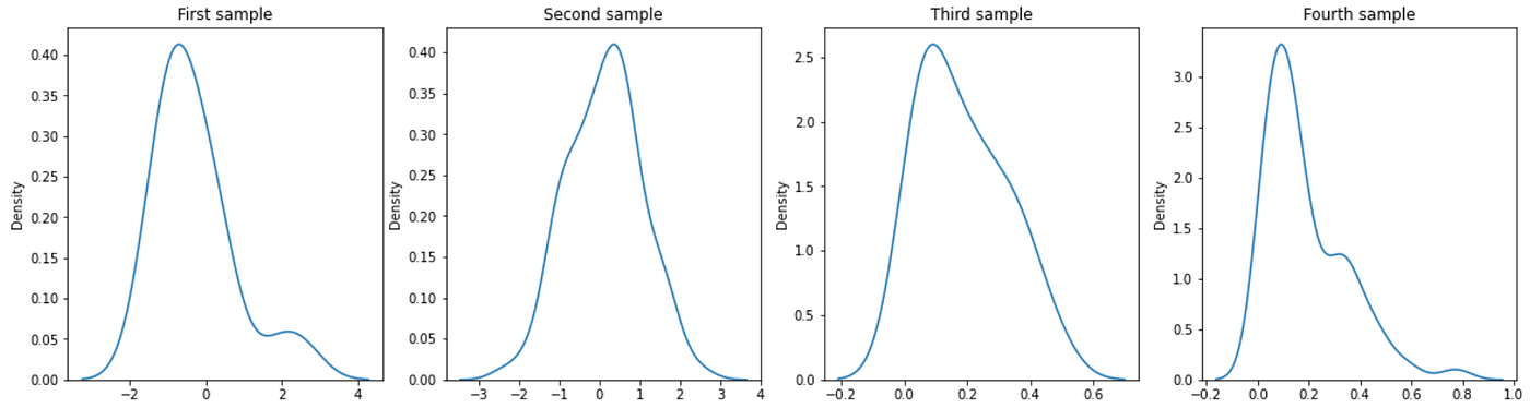
In precept, trying on the plots the normality assessments ought to reject the null speculation for the fourth pattern, and mustn’t reject it for the second pattern. Alternatively, Outcomes for the primary and the third samples are troublesome to evaluate by simply trying on the plots.
Shapiro-Wilk check
Right here is the implementation of the Shapiro-Wilk check:
Pattern 1: ShapiroResult(statistic=0.869, pvalue=0.011)
Pattern 2: ShapiroResult(statistic=0.996, pvalue=0.923)
Pattern 3: ShapiroResult(statistic=0.926, pvalue=0.134)
Pattern 4: ShapiroResult(statistic=0.878, pvalue=1.28e-11)
Outcomes present that we might reject the null speculation (the samples don’t comply with a traditional distribution) for samples 1 and 4.
Kolmogorov–Smirnov check
Right here is the implementation of the Kolmogorov–Smirnov check:
Pattern 1: KstestResult(statistic=0.274, pvalue=0.081)
Pattern 2: KstestResult(statistic=0.091, pvalue=0.070)
Pattern 3: KstestResult(statistic=0.507, pvalue=2.78e-05)
Pattern 4: KstestResult(statistic=0.502, pvalue=4.51e-47)
Outcomes present that we might reject the null speculation (the samples don’t comply with a traditional distribution) for all of the samples.
Since any such check can be relevant to any sort of distribution, we will evaluate the samples between them.
Samples 1 and a pair of: KstestResult(statistic=0.32, pvalue=0.039)
Samples 3 and a pair of: KstestResult(statistic=0.44, pvalue=0.001)
Samples 4 and a pair of: KstestResult(statistic=0.44, pvalue=2.23e-17)
D’Agostino-Pearson’s K² check
Right here is the implementation of the D’Agostino-Pearson’s K² check:
Pattern 1: NormaltestResult(statistic=10.13, pvalue=0.006)
Pattern 2: NormaltestResult(statistic=0.280, pvalue=0.869)
Pattern 3: NormaltestResult(statistic=2.082, pvalue=0.353)
Pattern 4: NormaltestResult(statistic=46.62, pvalue=7.52e-11)
Equally to the Shapiro-Wilk check, outcomes present that we might reject the null speculation (the samples don’t comply with a traditional distribution) for samples 1 and 4.
Testing the normality of a pattern is important to satisfy the assumptions of most of the hottest statistical assessments. Nonetheless, there are various normality assessments within the literature that make it troublesome to find out which is probably the most appropriate normality.
Due to this fact, this text has described the three essential normality assessments ((1) Shapiro-Wilk, (2) Kolmogorov–Smirnov, and (3) D’Agostino-Pearson’s K²) and has carried out them on 4 completely different samples.
Each the present literature and the outcomes of the experiment result in conclude that, normally, the advisable check to make use of is the Shapiro-Wilk [5].
[1] ReseatchGate, A Comparability amongst Twenty-Seven Normality Checks
[2] Actual statistics, Shapiro-Wilk Authentic Check
[3] Statistics How To, Kolmogorov-Smirnov Goodness of Match Check
[4] Actual statistics, D’ Agostino-Pearson Check
[5] Nationwide Library of Medication, Normality Checks for Statistical Evaluation: A Information for Non-Statisticians
