Visualizing sea ice focus with scatter plot and warmth map
Local weather change, a worldwide phenomenon, impacts Earth’s climate patterns. It produces penalties akin to deserts increasing and warmth waves changing into extra frequent. The elevated temperature within the Arctic has additionally contributed to melting permafrost and sea ice loss.
Let’s speak in regards to the sea ice. Polar amplification is a phenomenon by which the temperature close to the Earth’s pole is enchanted higher than the remainder of the globe. This resulted within the lack of sea ice previously a long time.
To deal with the issues, there are efforts worldwide to decelerate local weather change. Monitoring and recording are strategies that assist us analyze the change course of. This text will present two graphs, a scatter plot and a warmth map, to visualise the ocean ice focus with Python.
Let’s get began
The downloaded dataset is known as “Sea ice focus day by day gridded information from 1979 to current derived from satellite tv for pc observations” (hyperlink) Copyright © (2022) EUMETSAT. The time of the dataset is from January 2010 to December 2021, 12 years in whole, from the Copernicus web site.
The product used is the World Sea Ice Focus Local weather Knowledge Document produced by the European Organisation for the Exploitation of Meteorological Satellites Ocean and Sea Ice Satellite tv for pc Software Facility (EUMETSAT OSI SAF).
To get the dataset, I adopted the insightful steps from these 2 articles:
- Learn ERA5 Straight into Reminiscence with Python (hyperlink)
- Finest free API for climate information: ERA5! (hyperlink)
All mental property rights of the OSI SAF merchandise belong to EUMETSAT. Extra details about the dataset possession, copyright, acknowledgment, and quotation may be discovered right here: hyperlink and right here: hyperlink.
After downloading to your pc, I like to recommend saving the recordsdata in a folder for simply importing within the subsequent step.
The netCDF4 library is for studying the downloaded recordsdata in NetCDF (Community Widespread Knowledge Kind) format. The full file dimension that we’re going to work with is kinda large. Thus, it can take a while to course of. The tqdm library can present us progress bars.
To learn the recordsdata, we have to know the recordsdata’ names. The next code is used to get each file title within the folder the place they’re saved.
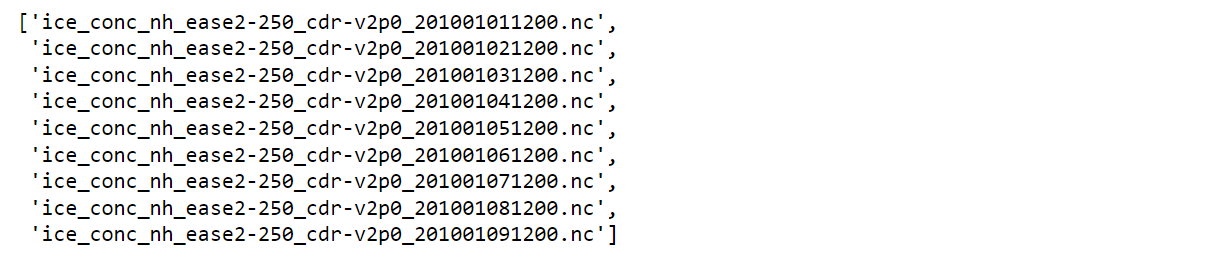
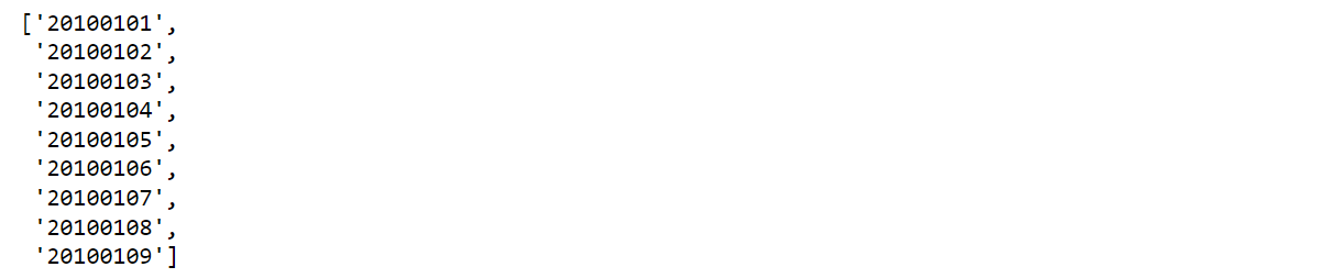
It may be seen that the file names comprise the date stamp. This can be utilized for assigning the dates to every dataset. Create a listing of dates.
Discover information
Earlier than persevering with, let’s discover the variables that every file comprises.
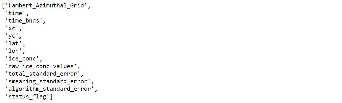
For extra info, use the code under to get extra element from every variable.
To visualise the ocean ice focus, three variables can be used:
- lat: latitude
- lon: longitude
- ice_conc: filterssea_ice_area_fraction; totally filtered focus of sea ice utilizing atmospheric correction of brightness temperatures and open water
Create DataFrame
We’ll learn the NetCDF recordsdata and switch them right into a DataFrame for working with Python. Outline capabilities for shortly making a DataFrame.
Apply the capabilities. Solely the proportion concentrations above 50 are chosen to keep away from extreme information. By the best way, the quantity may be modified.

Observe: If an error in regards to the reminiscence reveals up, I like to recommend doing a listing slicing. Dividing the info into two or three elements to work with small information and saving the output DataFrame with DataFrame.to_csv. Repeat the method till full the record. After that, learn each DataFrame and concatenate them with pandas.concat.
This text will primarily give attention to the ice sea above the Arctic Circle, 66°N roughly. If you’re within the ice sea under the Antarctic Circle, the latitude worth within the code under may be modified. Filter the DataFrame and group by the yr and month.
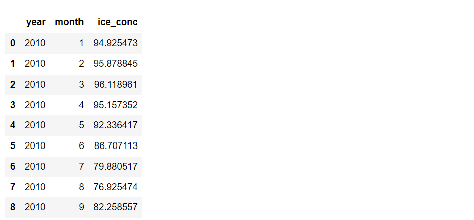
Plot a Time-series graph from the DataFrame.

The strains within the time-series graph present that August is the month when the typical share focus reaches the bottom level. This is smart since it’s Summer time within the northern hemisphere.
This text will information learn how to visualize the info utilizing a scatter plot on polar axis and a warmth map.
Earlier than persevering with, the obtained DataFrame will not be prepared for plotting. The latitude is required to be scaled from [66,90] to [0,1] to facilitate the info visualization. Furthermore, the longitude vary comprises unfavourable values from [-180,180], that are wanted to show right into a optimistic vary. Let’s outline a perform to transform the values.
Create a listing of years and months to filter the DataFrame.
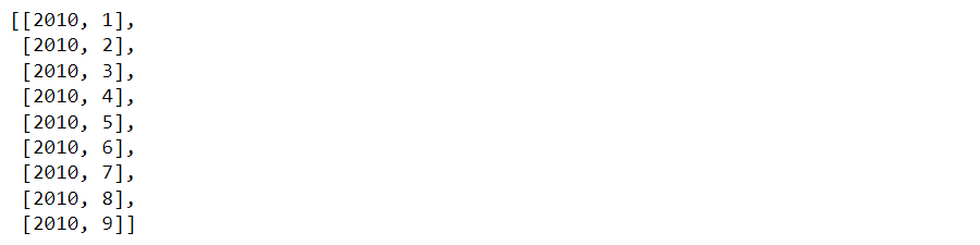
The subsequent step is making use of the perform and filtering with the record of years and months.

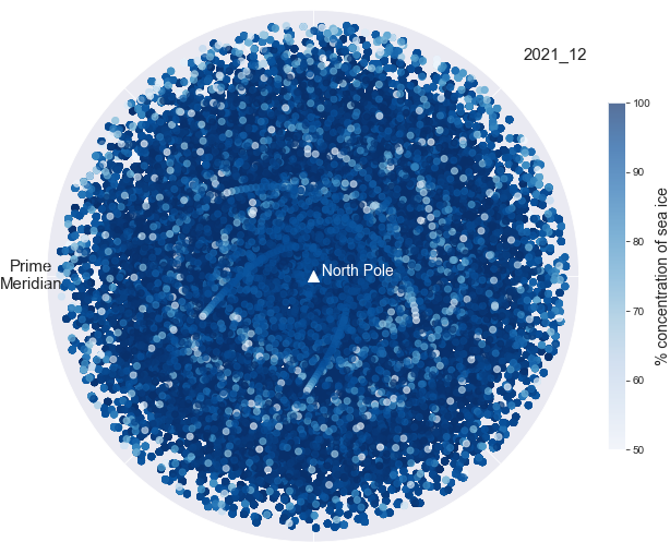
Scatter plot on polar axis
The concept is to look from above the North Pole. Thus, we’re going to plot the scatter plot on the polar axis to simulate the viewpoint. Observe that the outcomes can be saved to your pc to be used later.

Create a GIF file
Making an animation is another thought for making the plots look fascinating. Thus, let’s mix the plots and switch them right into a GIF file. For instance, I’ll mix the scatter plots from each month in 2020 and 2021.
Voila!!….

From the saved output, we are able to create a GIF file choosing solely the identical month to match annually’s information. For instance, the next code reveals learn how to mix each plot of September.
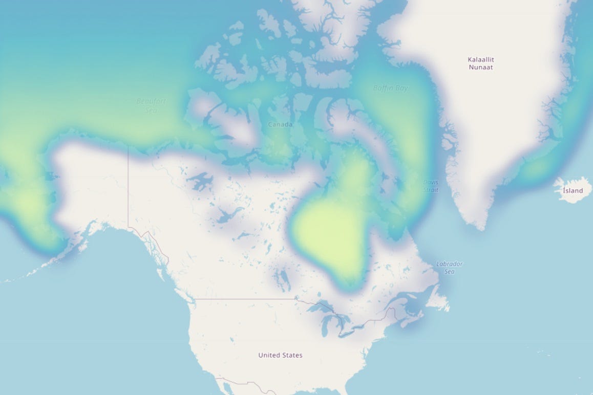
Warmth map
To create a warmth map over the world map, Folium is a robust Python library for working with geospatial information. Begin with importing the libraries.
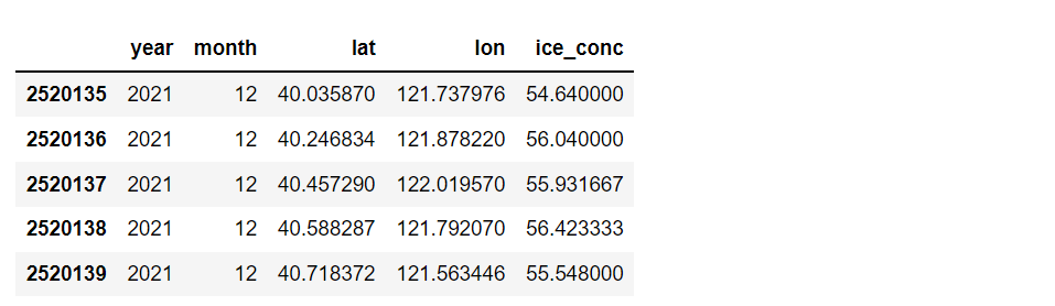
We have to put together the info earlier than making use of with Folium. This time the entire information above the Equator line is chosen. After that, carry out groupby and calculate the month-to-month common. Then, select the month to plot. For instance, the dataset under is from December 2021.
From the DataFrame, create a listing of knowledge and colours for plotting.
Plot a Warmth map with the Folium library.

Warmth map with time
Folium additionally has a perform referred to as HeatMapWithTime for creating an animation by combining a number of warmth maps. I’ll plot the warmth maps from January 2019 to December 2021, 24 months.
Plot the info with HeatMapWithTime.

Abstract
This text has proven a sea ice information supply and learn how to import and put together the info. The 2 graphs for visualizing sea ice focus are the scatter plot on polar axis and the warmth map. The 2 graphs may be improved by creating animation to make the outcomes look fascinating.
This text primarily focuses on the ocean ice above the Arctic circle. By the best way, the strategy may be utilized to the ocean ice within the southern hemisphere, under the Antarctic circle.
You probably have any recommendations or questions, please be happy to remark.
Thanks for studying
