
The right way to use inverse rework sampling to enhance your mannequin
Normalizing knowledge is a typical activity in knowledge science. Typically it permits us to hurry up gradient descent or enhance mannequin accuracy, and in some circumstances it completely essential. For instance, the mannequin I described in my final article can’t deal with targets which might be distributed non-normally. Some normalization methods, like taking a logarithm, may go more often than not, however on this case, I made a decision to attempt one thing that may work for any knowledge, regardless of the way it was initially distributed. The tactic I’ll describe beneath relies on inverse rework sampling: the principle thought is to assemble such operate F, primarily based on the info’s statistical properties, so F(x) is distributed usually. Right here’s the best way to do it.
The algorithm I’m speaking about relies on the inverse rework sampling technique. This technique is extensively utilized in pseudo-random quantity turbines to generate numbers from any given distribution. Having uniformly distributed knowledge you possibly can at all times rework it into distribution, with any given cumulative density operate (or CDF for brief). A CDF exhibits what quantity of information factors of distribution is smaller than a given worth and principally denotes all of the statistical properties of the distribution.
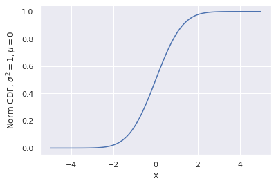
The principle thought is that for any constantly distributed knowledge xᵢ, CDF(xᵢ) is distributed uniformly. In different phrases, to get uniformly distributed knowledge one simply takes a CDF of every level. The mathematical proof of this assertion is out of the scope of this text, however the truth that stated operation is actually simply sorting all of the values and changing every worth with its quantity offers it an intuitive sense.

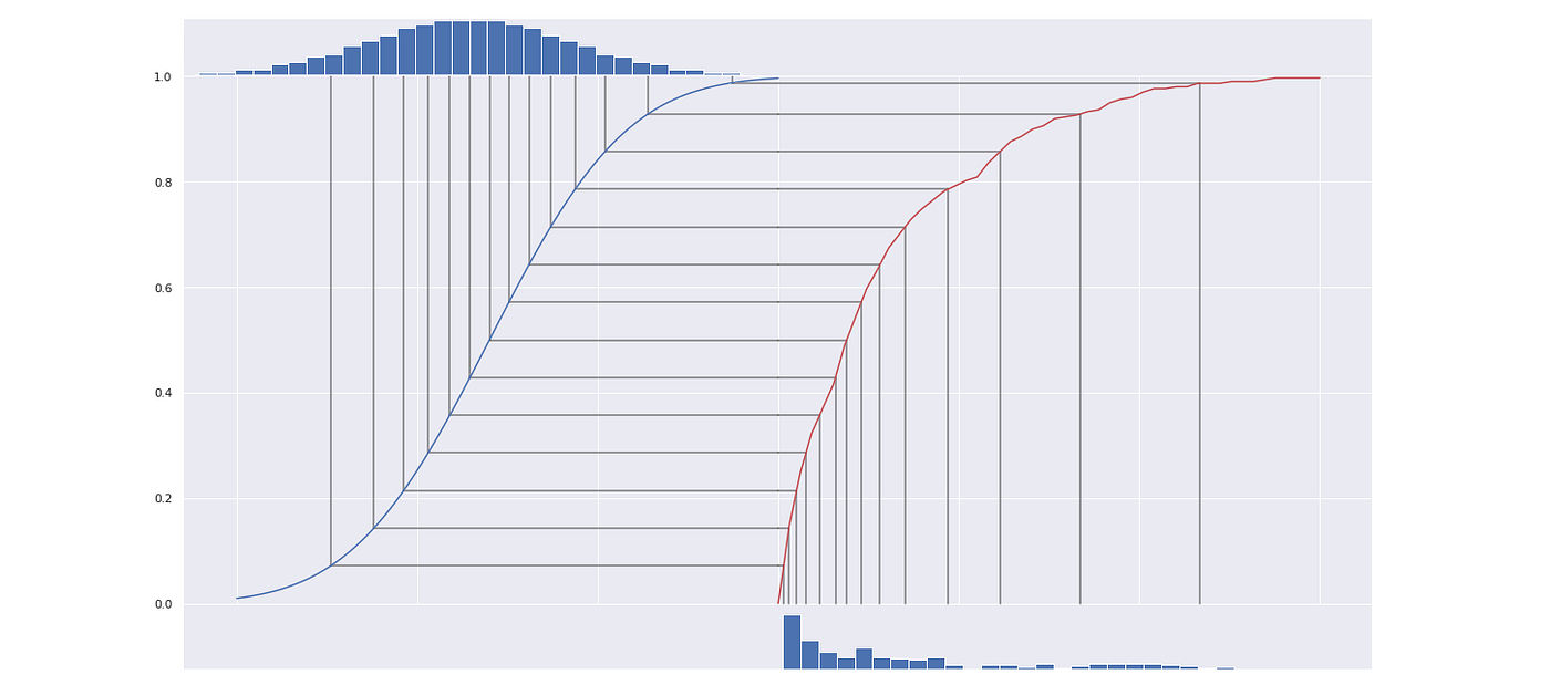
Within the gif above you possibly can see the way it works. I generated some messy distributed knowledge after which calculated its CDF (the crimson line) and remodeled the date with it. Now the info is uniformly distributed.
Calculating CDF is simpler than it appears. Bear in mind, a CDF is a fraction of information smaller than the given one.
def CDF(x, knowledge):
return sum(knowledge <= x) / len(knowledge)
It’s price mentioning {that a} CDF usually is a bijective operate, which signifies that the transformation is reversible. We are able to use this truth to rework obtained uniform distribution into any distribution we wish, say regular distribution. In an effort to try this we have to compute an inverse CDF of the distribution we need to get. Typically, it’s not the simplest activity. The operate we’d like is known as a p.c level operate, or PPF for brief. Fortunately for us, the PPFs of any main distribution are accessible via the SciPy library, and one doesn’t have to compute it themselves.
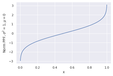
Right here’s the best way to interpret it: for any argument x between 0 and 1 PPF returns the utmost worth for the purpose to suit into x’th percentile. On the similar time being the inverse operate of a CDF it seems to be like a operate from the primary image, simply rotated 90°.
Now we have now a pleasant regular distribution as desired. Lastly, to make a operate that transforms our preliminary knowledge, all we have now to do to merge these two operations collectively into one operate:
from scipy.stats import normdef normalize(x, knowledge):
x_uniform = CDF(x, knowledge)
return norm.ppf(x_uniform)
The crimson line within the image above represents the ultimate rework operate.
By the best way, we are able to simply rework knowledge into every other distribution simply by changing PPF with one of many desired distribution. Right here is the transformation of our messy knowledge into lognormal distribution. Discover how the reworking curve is completely different.
Discover how the ultimate transformation is at all times monotonic. That signifies that no two factors are swapped after the transformation. If the worth of the preliminary characteristic is bigger for one level than for one more, after the transformation, the remodeled worth may even be larger for that time. This truth permits this algorithm to be utilized to knowledge science duties.
To sum up, not like extra frequent strategies, the algorithm described on this article doesn’t require any assumptions about preliminary distribution. On the similar time, the output knowledge follows the conventional distribution extraordinarily exactly. This technique has been proven to extend the accuracy of fashions, that assume enter knowledge distribution. For instance, the Bayesian mannequin from the final article has R² ~ 0.2 with out knowledge normalization and R² of 0.34 with normalized knowledge. Linear fashions have additionally proven enhancements in R² on 3–5 share factors on normalized knowledge.
That’s it. Thanks to your time, and I hope you discovered this text helpful!
