An Efficient Technique for Smaller Datasets

Ever since CNNs began to explode within the area of picture processing in 2012, these networks have been rapidly utilized to music style classification — and with nice success! At present, coaching CNNs on so-called spectrograms has grow to be state-of-the-art, displacing nearly all beforehand used strategies primarily based on hand-crafted options, MFCCs, and/or help vector machines (SVM).
Lately, it has began to indicate that including recurrent layers like LSTMs or GRUs to classical CNN architectures yields higher classification outcomes. An intuitive clarification for that is that the convolutional layers determine the WHAT and the WHEN, whereas the recurrent layer finds significant relationships between the WHAT and the WHEN. This structure is called a convolutional recurrent neural community (CRNN).

When studying about divide & conquer for the primary time, I used to be confused, as a result of I had heard of it in a army context. The army definition is
“to make a bunch of individuals disagree and combat with each other in order that they won’t be part of collectively in opposition to one” (www.merriam-webster.com)
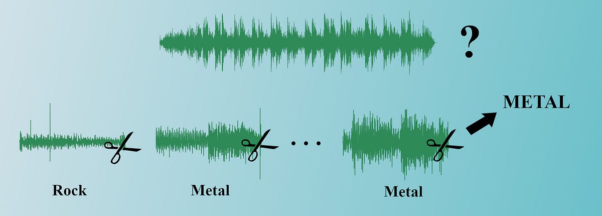
Nonetheless, that is nearly the other of its that means for our goal! See Desk 1, the place the three-step course of behind divide & conquer in pc science and music style classification is laid out.

Though the definitions are usually not the identical, they do overlap considerably, and personally, I discover the time period divide & conquer very becoming in each circumstances. In music style classification, the time period was first used (to my data) by Dong (2018). Nonetheless, different researchers like Nasrullah & Zhao (2019) have additionally used this methodology — simply not by the identical title.
Typically, style classification relies on precisely one 30-second snippet of a observe. That is partly as a result of generally used music knowledge sources just like the GTZAN or FMA datasets or the Spotify Internet API present tracks of this size. Nonetheless, there are three main benefits to making use of the divide & conquer method:
1. Extra Information
Given that you’ve got full-length tracks accessible, taking a 30-second slice and throwing away the remainder of a 3–4 minute observe could be very knowledge inefficient. Utilizing divide & conquer, a lot of the audio sign can be utilized. Furthermore, by permitting for overlap between slices, much more snippets could be drawn. In truth, I’d argue that this can be a type of pure and pretty seamless knowledge augmentation.
For instance, you will get greater than 80x the coaching knowledge from a 3-minute observe if you happen to draw 3-second snippets with an overlap of 1 second in comparison with drawing one 30-second snippet per observe. Even if you happen to solely have 30-second tracks accessible, you will get 14 snippets out of every of them with 3-second snippets and 1 second of overlap.
2. Decrease-Dimensional Information
A 30-second snippet produces fairly a big spectrogram. With widespread parameters, one spectrogram can have a form of (1290 x 120), i.e. over 150k knowledge factors. Naturally, a 3-second snippet with the identical parameters will produce a ~(129 x 120) spectrogram with solely 15k knowledge factors. Relying on the machine studying mannequin and structure you might be utilizing, this may scale back the mannequin complexity considerably.
Aspect observe: In case you might be unaware of what spectrograms are or why and the way they’re used for audio classification, I like to recommend this text by The Experimental Author for a pleasant and intuitive clarification.
3. Detached to Audio Enter Size
If you wish to apply your educated mannequin in the actual world, you’ll encounter tracks of all lengths. As a substitute of getting to wrestle with discovering simply the correct 30-second snippet to extract from it, you simply begin drawing 3-second snippets till the entire observe is roofed. And what if the enter observe is lower than 30 seconds lengthy? Is your mannequin strong sufficient to cope with 10-second jingles that are zero-padded to achieve 30 seconds? With divide & conquer, that is no situation.
Disadvantages
There are three main downsides to utilizing divide & conquer. Firstly, it provides further processing steps to separate the audio information and to carry out the aggregated predictions for a full observe. Furthermore, the snippet-based method requires a track-wise train-validation-test break up to keep away from intercorrelated training-, validation-, and check datasets.
Fortunately, each of those steps are already included in my single-label audio processing pipeline SLAPP, which is freely accessible on GitHub.
Lastly, the person snippet predictions are normally aggregated utilizing some form of majority vote. With that, your mannequin is totally oblivious to any musical relationships which unfold over greater than, e.g., 3 seconds of audio. That’s until you develop one other complicated meta classifier for the aggregation course of.
When to Use Divide & Conquer
In case you both have a lot of knowledge and require no extra of it or if you wish to analyze musical constructions which unfold over longer time frames, chances are you’ll not wish to use a divide & conquer method. Nonetheless, if in case you have restricted knowledge and wish to construct a sturdy and versatile classifier with it, do contemplate this thrilling and efficient method!

What’s SLAPP?
This text additionally serves as a showcase for my newly developed single-label audio processing pipeline (SLAPP). This device automates your entire knowledge processing workflow for single-label audio classification duties. This consists of splitting the tracks into snippets, computing spectrograms, performing a track-wise train-validation-test break up, and rather more.
Since processing audio knowledge takes a extremely very long time on a house pc, SLAPP lets you shut down your pc at any time and reload your progress with none important lack of time or knowledge. After having developed this pipeline for my bachelor’s thesis, I attempted it out on a few classification duties and had nice enjoyable and success with it.
Take a look at SLAPP on GitHub and check out it out for your self.
Utilizing SLAPP to Course of GTZAN
GTZAN is a widely known and publicly accessible dataset for style classification, that includes 100 30-second-long tracks from 10 totally different genres. This dataset is ideal for our functions as a result of there’s a enormous physique of analysis behind it and since it solely has a restricted quantity of information.
To be able to use SLAPP, you must place your MP3 (not WAV) information in a folder construction similar to the one proven in Determine 1.

Since GTZAN is available in precisely such a folder construction (yay!), all we have to do now could be to transform the WAV information into MP3 information and we are able to get began. I recommend you do that by looping by way of the listing and copying every file into a brand new listing with the identical construction utilizing
from pydub import AudioSegmentAudioSegment.from_wav("/enter/file.wav").export("/output/file.mp3", format="mp3")
Subsequent, all you must do is clone the SLAPP repository by navigating into your required listing and utilizing:
git clone https://github.com/MaxHilsdorf/single_label_audio_processing_pipeline
Be sure that your system fulfills all the necessities to make use of SLAPP; as an illustration, the Python libraries Pydub and Librosa in addition to the audio codec FFmpeg (described intimately within the repository).
Now, inside SLAPP, we open “pipeline_parameters.json” and set the parameters like this:
This fashion, we extract as much as 14 3-second slices from every 30-second observe inside GTZAN, permitting for an overlap of 1 second. By working “build_dataset.py”, the dataset is constructed, and by working “process_dataset.py”, the dataset is then normalized and shuffled. That’s all you must do. SLAPP takes care of the remainder for you.
With validation- and check splits of 10% every, you’ll get hold of 11,186 coaching spectrograms and 1,386 spectrograms for each, validation- and check knowledge. Every spectrogram has a form of (130 x 100).
Aspect observe: If you’re not simply studying alongside, however truly coding alongside, this processing step will take some time, as a result of there are many computational steps. At any time throughout the course of, you possibly can cease the scripts and relaunch them to renew the place you left off. In case you expertise any technical points with SLAPP, be happy to let me know, since that is my first software program launch and it could have a lot of bugs or my documentation could also be inadequate.

Mannequin Constructing
Utilizing the Keras library, I constructed a CRNN like this:
The concept behind this CRNN structure is to make use of convolutional layers + max pooling to squeeze the frequency dimension to a scalar worth whereas holding the time dimension as a vector. This enables us to use a gated recurrent unit (GRU) to the options extracted by the convolutional blocks. The sort of structure was (to my data) launched by Choi et al. (2017) and has been adopted in a number of research, as an illustration by Nasrullah & Zhao (2018) and Bisharad & Laskar (2019).
See Determine 2 for an in depth overview of the structure used.

Within the growth part, I attempted out totally different variations of this structure and in contrast the validation loss between these fashions. This specific mannequin achieved prime outcomes with solely ~400k parameters.
Aspect Observe: SLAPP will, on this case, provide you with a coaching knowledge tensor of form (11186, 100, 130). Nonetheless, to coach this particular CRNN, the enter must be reshaped to (11186, 130, 100, 1), successfully swapping the time- and frequency axes (numpy.swapaxes) and including one other dimension (numpy.expand_dims).
Mannequin Coaching
I educated the mannequin with Adam optimizer, a studying charge of 0.0001, categorical cross-entropy loss, and a batch measurement of 32. Moreover, I used the EarlyStopping, ReduceLROnPlateau, and ModelCheckpoint callbacks offered by Keras to make sure clean coaching and that solely the most effective mannequin is saved.
As you possibly can see in Determine 3, the coaching metrics attain precision and recall scores near 90%, whereas the validation precision and recall scores converge someplace between 62 and 73%. Seeing as we’re dealing solely with 3-seconds of audio and 10 balanced lessons ( → 10% accuracy by way of random guessing), that is already fairly spectacular. Total, the most effective mannequin on this coaching run achieved a validation accuracy of 67.32%.

To realize extra secure outcomes, 10 coaching runs have been began and evaluated to acquire imply scores and commonplace deviations for the metrics of curiosity. Remember the fact that this text doesn’t intention to supply a classy statistical analysis, however moderately to indicate the effectiveness of divide & conquer classification utilizing an instance.

How one can Compute Observe-Primarily based Predictions?
For the track-based predictions, I loaded every observe within the check dataset as an MP3 file. The check observe names are routinely written to “train_val_test_dict.json” in your knowledge listing by SLAPP. From there, the process I used is the next:
- Break up the observe into as many snippets as potential (3-second snippets with 2 sec overlap on this case).
- Remodel every snippet right into a mel spectrogram that fits the enter form of the educated mannequin.
- Get the uncooked class predictions for every snippet.
- Sum the uncooked scores for every class throughout all snippets.
- Your international prediction is the category with the highest rating sum.
Since this may get fairly difficult for freshmen, I’m going to give you one other module that automates this track-based prediction course of: Please discover the module and its documentation right here.
Classification Outcomes
I educated and evaluated the mannequin described above ten occasions and averaged the accuracy scores to do away with among the randomness of the method.
See Determine 4 for a visible overview of the accuracy scores obtained. The very first thing we discover is that the mannequin carried out roughly equally effectively on the validation- and check knowledge, which is an efficient signal. Additional, all commonplace deviations are actually small, which tells us that we are able to actually on variations in imply accuracy.
It’s simple to see that the track-based classification outperformed the snippet-based classification by a mean distinction of ~12.2 proportion factors. Whereas we’re not going to do any statistical assessments for the sake of simplicity, it’s simple that the track-based classification by way of divide & conquer is superior on this case.

What If We Had Used The Full 30-second Snippets?
Thus far, now we have proven that (on this instance) the track-based divide & conquer classification outperforms the 3-second single-snippet classification. Nonetheless, possibly we might have achieved a a lot greater accuracy if we had constructed a CRNN on the 1000 30-second audio slices in “uncooked” GTZAN.
That’s potential, so I attempted it out. I constructed one other CRNN of the same structure (though ~half the parameters as a result of there’s much less knowledge) primarily based on 30-second slices and educated it 10 occasions to common the accuracy scores obtained. This methodology averages out at an accuracy of solely 55.8% (SD=0.043), underperforming any of the 3-second fashions by a big margin.

Divide & Conquer Does In Truth Conquer
This text exhibits how a divide & conquer method will help to construct a powerful classifier for audio classification issues even when not a lot coaching knowledge is current. The info processing pipeline SLAPP makes it very easy to carry out the processing steps crucial to construct a divide & conquer classifier for single-label audio classification duties.
3 Seconds are Higher Than 30 Seconds
How come 30-second slices are even worse than 3-second slices though they maintain extra data? Evidently rising the dataset measurement by drawing 3-second slices helps the mannequin to extract significant options, whereas it appears to get misplaced when coping with a extremely small dataset consisting of giant spectrograms.
Arguably, if different knowledge codecs like MFCCs or hand-crafted options with a smaller dimensionality had been used, the mannequin would have dealt extra simply with the 30-second audio information. Nonetheless, this text goes to indicate that just about any audio dataset could be categorised with spectrogram knowledge — if divide & conquer is used.
Different Functions of SLAPP + Divide & Conquer
If you wish to strive the proposed methodology on one other related drawback, listed below are some concepts which will encourage your subsequent knowledge science undertaking:
- Intercourse recognition primarily based on speech knowledge
- Accent recognition primarily based on speech knowledge
- Emotion classifier for music
- Constructing classifiers utilizing audio knowledge from machine sensors
Thanks very a lot on your curiosity in my work! Please let me know if something isn’t working for you or if in case you have hassle understanding or making use of the ideas.
[1] Bisharad, D. & Laskar, R. H. (2019). Music Style Recognition Utilizing Convolutional Recurrent Neural Community Structure. In: Knowledgeable Methods 36,4.
[2] Choi, Okay.; Fazekas, G.; Sandler, M. & Cho, Okay. (2017). Convolutional Recurrent Neural Networks for Music Classification. In: Worldwide Convention on Acoustics, Speech, and Sign Processing 2017.
[3] Dong, M. (2018). Convolutional Neural Community Achieves Human-level Accuracy in Music Style Classification. In: Convention on Cognitive Computational Neuroscience, 5–8 September 2018, Philadelphia, Pennsylvania.
[4] Nasrullah, Z. & Zhao, Y. (2019). Music Artist Clasification from Audio, Textual content, and Pictures Utilizing Deep Options. In: arXiv, DOI: 10.48550/arXiv.1707.04916
