Modeling Advertising Combine Utilizing Smoothing Splines | by Slava Kisilevich | Jul, 2022

Capturing non-linear promoting saturation and diminishing returns with out explicitly reworking media variables

The established method amongst entrepreneurs for modeling advertising and marketing combine is to use linear regression fashions which assume the connection between advertising and marketing actions resembling commercial spend and the response variable (gross sales, income) is linear. Previous to modeling, media spend variables ought to bear two crucial transformations to correctly seize the carryover impact and the saturation impact of the commercial spend. It’s identified, that commercial spend will not be linear with respect to the response variable and follows the legislation of diminishing returns. Nevertheless, the useful type of the saturation curve will not be identified prematurely. Subsequently, the modeler ought to first hypothesize in regards to the potential transformation capabilities that ought to be utilized to every media exercise channel to match the true spend-to-response relationship. On this article, I present an alternate method to modeling advertising and marketing combine through the use of Smoothing Splines, which is the way in which to mannequin the non-linear relationship between dependent and unbiased variables throughout the framework of a linear mannequin. By following this method, the mannequin will set up the non-linear relationship between media exercise variables and the response variable with out the necessity to rework these unbiased variables to account for the non-linear relationships.

The instinct behind the transformation of media exercise variables

Let’s perceive by instance why the transformation of media exercise variables is a crucial step within the framework of a linear mannequin.

I generate a media variable with commercial spend whose saturation impact is described by the hill perform with two parameters γ, controlling the inflection level, and α the form of the curve.

import numpy as np
spend = np.random.rand(1000, 1).reshape(-1)
noise = np.random.regular(measurement = 1000, scale = 0.2)#hill transformation
alpha = 2
gamma = 0.1spend_transformed = spend**alpha / (spend ** alpha + gamma ** alpha)response = 1 + 3 * spend_transformed  +  noise

For an outline of various transformation capabilities that can be utilized for modeling saturation results and diminishing returns you might test the next article:

Let’s plot the spend-to-response relationship:

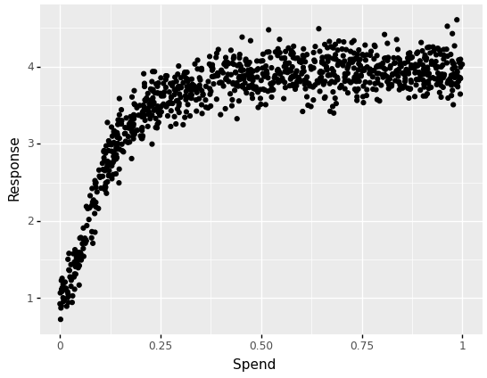
Now, what occurs once we match a linear regression mannequin with out first reworking our unbiased variable?

import statsmodels.api as sm
spend_with_intercept = sm.add_constant(spend)
ols_model = sm.OLS(response, spend_with_intercept)
ols_results = ols_model.match()
ols_results.params

As anticipated, the linear regression will not be capable of seize the non-linear relationship. Now, in a real-life state of affairs, at this second, we’ve got to resolve on the transformation perform and its parameters. Let’s rework our spend variable utilizing the hill perform with barely completely different parameters that have been used to simulate the response variable and match the linear regression mannequin.

alpha = 2
gamma = 0.3#hill transformation
spend_transformed = spend**alpha / (spend ** alpha + gamma ** alpha)X_hill_transformed = sm.add_constant(spend_transformed)
ols_model_hill_transformed = sm.OLS(response, X_hill_transformed)
ols_results_hill_transformed = ols_model_hill_transformed.match()
ols_results_hill_transformed.params

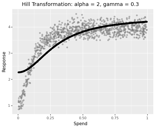
The mannequin now captures non-linearities however within the area of decrease spendings, there’s an apparent mismatch. Let’s attempt once more with completely different parameter values.

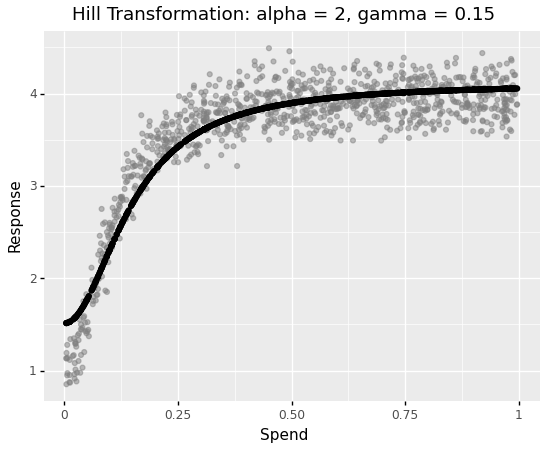
As we transfer the gamma worth nearer to the unique worth used to generate the response, we get a greater and higher match. After all, the modeler doesn’t attempt completely different parameters manually. As an alternative, this course of is automated by hyperparameter optimization frameworks. Nevertheless, the transformation step nonetheless requires effort to agree upon the right transformation perform and computing time to seek out the approximate transformation parameters to higher match a mannequin to information.

Is there a strategy to omit the transformation step and let the mannequin discover the non-linear relationships? Sure. In one among my earlier articles, I described a machine-learning method to reaching this:

Regardless of some great benefits of utilizing arbitrary tree-based machine studying algorithms that enhance accuracy over linear regression approaches and take care of non-linearities, one of many essential disadvantages is that these algorithms don’t keep a lot interpretability as linear fashions do. So further approaches like SHAP are wanted to be utilized to elucidate media efficiency, which is probably not intuitive to the entrepreneurs. The second method is to increase linear fashions in such a approach that permits to:

• Keep the interpretability
• Mannequin the non-linear results

Such an extension is named Generalized Additive Fashions the place modeling of non-linear results is achieved through the use of the so-called Smoothing Splines.

An summary of Generalized Additive Fashions (GAM) and Smoothing Splines

The usual (additive) linear mannequin takes the next type

the place betas are coefficients and epsilon is the error time period.

The generalized additive mannequin extends linear regression with the next type:

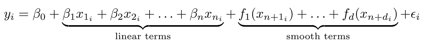
the place f is a clean perform. Primarily GAM provides the sum of smoothing phrases to the sum of linear phrases. There are fairly a couple of approaches for smoothing capabilities of which penalized smoothing splines are really helpful for his or her computational effectivity.

The penalized smoothing splines work as follows:

First, the vary of information variables is split into Okay distinct areas having Okay area boundaries referred to as knots. Second, inside every area, low-degree polynomial capabilities are fitted to the info. These low-degree polynomials are referred to as foundation capabilities. The spline is a sum of weighted foundation capabilities, evaluated on the values of the info. A penalty is added to the least sq. loss perform to regulate the mannequin’s smoothness. The smoothing parameter lambda controls the trade-off between the smoothness and wiggliness of the estimated smoothing perform f. Low values of lambda end in an un-penalized spline, whereas excessive values of lambda end in a linear line estimate.

Generalized Additive Fashions in Python

Let’s return to the earlier instance and match the penalized smoothing splines to the spend-response information.

In Python, pyGAM is the bundle for constructing Generalized Additive Fashions

pip set up pygam

I mannequin the linear GAM utilizing the LinearGAM perform. The spline time period is outlined through the use of an s perform which expects an index of the variable. n_splines controls what number of foundation capabilities ought to be fitted. I set lambda to a really low worth of 0.1 which implies I nearly don’t penalize the wiggliness of the spline

from pygam import LinearGAM, s
gam_hill = LinearGAM(s(0, n_splines=10), lam = 0.1).match(spend, response)

Let’s perceive the output of the mannequin:

gam_hill.abstract()

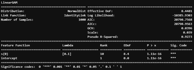
The essential components value mentioning are:

• Rank — variety of splines or foundation capabilities
• Lambda — the smoothing parameter
• EDoF — efficient levels of freedom. Larger EDoF suggests extra advanced splines. When EDoF is near 1, it means that the underlined time period is linear. The documentation of mgcv bundle in R (an equal of pyGAM) suggests the next rule of thumb for the choice of quite a few splines:
  As with all mannequin assumptions, it’s helpful to have the ability to test the selection of n_splines informally. If the efficient levels of freedom for a mannequin time period is estimated to be a lot lower than n_splines-1 then that is unlikely to be very worthwhile, however because the EDoF approaches n_splines-1, checking may be essential: enhance the n_splines and refit the unique mannequin. If there aren’t any statistically essential adjustments on account of doing this, then n_splines was massive sufficient. Change within the smoothness choice criterion, and/or the efficient levels of freedom, when n_splines is elevated, present the apparent numerical measures for whether or not the match has modified considerably.

Let’s extract the spend part:

XX = gam_hill.generate_X_grid(time period=0, n = len(response))
YY = gam_hill.partial_dependence(time period=0, X=XX)

The anticipated worth of the response is the sum of all particular person phrases together with the intercept:

intercept_ = gam_hill.coef_[-1]
response_prediction = intercept_ + YY

Let’s plot the ultimate spend-to-response relationship:

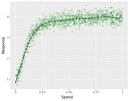
The mannequin might seize the non-linear spend-to-response relationship with out reworking the unbiased variable.

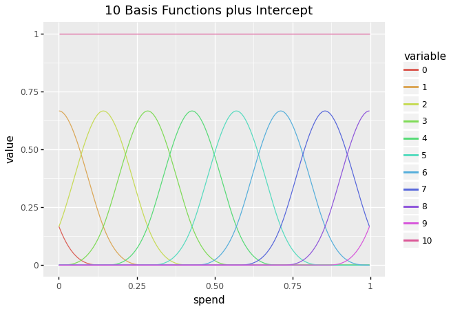
For completeness, let’s check out the idea capabilities of the spline:

basis_functions = pd.DataFrame(gam_hill._modelmat(spend).toarray())
basis_functions["spend"] = spend#plot
ggplot(pd.soften(basis_functions, id_vars="spend"), aes("spend", "worth", group="variable", colour = "variable")) + geom_line() + ggtitle(f"{len(basis_functions.columns) - 2} Foundation Capabilities plus Intercept")

The ensuing spline is a weighted sum of foundation capabilities multiplied by their corresponding coefficients:

foundation = gam_hill._modelmat(spend).toarray()  
coefficients = gam_hill.coef_#omit intercept
spline = foundation[:,:-1] @ coefficients[:-1]

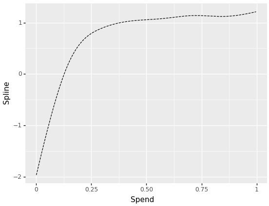
I omitted the addition of the intercept, so the plot exhibits a decomposed smoothing impact of the spend variable.

Now, once we perceive how GAM works, I present how it may be integrated into the MMM framework. I’ll reuse the framework I launched within the following paper:

The adjustments are minimal. As an alternative of Random Forest, I’m utilizing GAM. The SHAP part which was crucial to elucidate black-box fashions will not be wanted anymore. Due to the linear additivity of parts in GAM, we analyze the consequences of every smoothed media variable nearly equally as in linear regression fashions.

Knowledge

As in my earlier articles on MMM, I proceed utilizing the dataset supplied by Robyn beneath MIT Licence for benchmarking and observe the identical information preparation steps by making use of Prophet to decompose tendencies, seasonality, and holidays.

The dataset consists of 208 weeks of income (from 2015–11–23 to 2019–11–11) having:

• 5 media spend channels: tv_S, ooh_S, print_S, facebook_S, search_S
• 2 media channels which have additionally the publicity data (Impression, Clicks): facebook_I, search_clicks_P (not used on this article)
• Natural media with out spend: e-newsletter
• Management variables: occasions, holidays, competitor gross sales (competitor_sales_B)

The evaluation window is 92 weeks from 2016–11–21 to 2018–08–20.

Modeling

The modeling steps are precisely the identical as I described within the earlier article:

I’ll point out the essential adjustments with respect to GAM.

pyGAM expects fairly a non-standard definition of enter options. I’ve written a helper perform that takes two forms of options: those who ought to be modeled as linear and those who ought to be modeled as smoothing splines. As well as, the variety of splines is supplied as a parameter

def build_gam_formula(information, 
base_features, 
smooth_features, 
n_splines = 20):
#set the primary spline time period
channel_index = information.columns.get_loc(smooth_features[0])
method = s(channel_index, 
n_splines, 
constraints='monotonic_inc')
for smooth_channel in smooth_features[1:]:
channel_index = information.columns.get_loc(smooth_channel)        #clean time period
method = method + s(channel_index, 
n_splines, 
constraints='monotonic_inc')    for base_feature in base_features:
feature_index = information.columns.get_loc(base_feature)        #linear time period
method = method + l(feature_index)return method

The ensuing method utilized to six media channels and 5 management variables appears like this:

s(5) + s(6) + s(7) + s(8) + s(9) + s(10) + l(0) + l(1) + l(2) + l(3) + l(4)

s(5) for instance means making use of smoothing splines on the variable whose column index within the information set is 5.

Take note of the constraints parameter with the worth monotonic_inc. Within the context of linear regression, we apply some agreed-upon enterprise logic associated to the saturation impact and diminishing returns by constraining linear coefficients to be optimistic in order that a rise in commercial spend is not going to trigger a lower in response.

Verify this text for extra particulars:

Within the context of GAM, I put a constraint on smoothing splines to be monotonically growing.

Parameter Optimization

Together with 5 adstock parameters, I optimize the smoothing parameter lambda within the vary between 0.1 and 1000 for all variables. Word: it isn’t fairly clear to me why pyGAM requires smoothing parameters for variables which are explicitly outlined as linear.

Last Mannequin

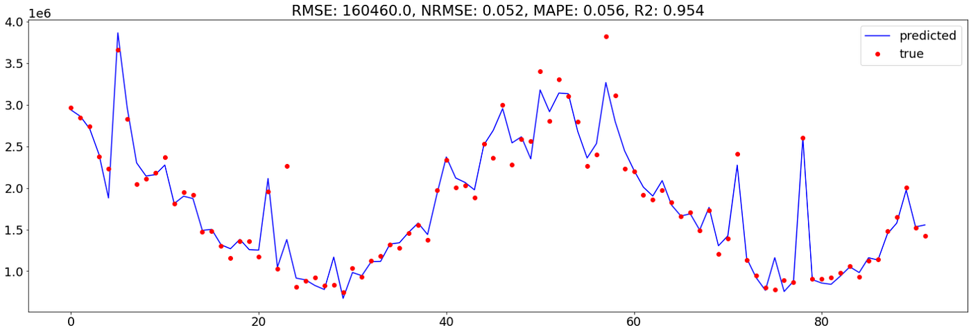
I constructed the ultimate mannequin utilizing the window of 92 weeks. The abstract of the mannequin is proven beneath:

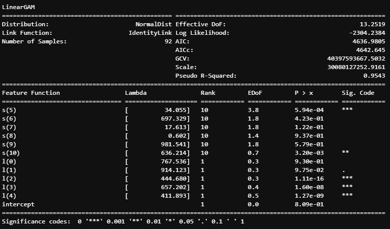
The abstract exhibits that 3 out of 6 media channels received a excessive smoothing lambda, and their corresponding EDoF close to 1 suggests an nearly linear relationship.

If evaluating error metrics to the evaluations, GAM achieved increased accuracy than the Bayesian method and barely decrease than the Random Forest

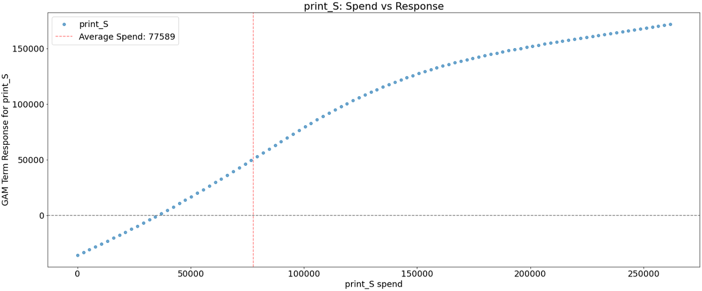
Diminishing return / Saturation impact

Let’s plot the ensuing spend-to-response relationship. The vertical line corresponds to the common spend within the channel. The x-axis is the media spend. The y-axis is the impact of spend on the response variable

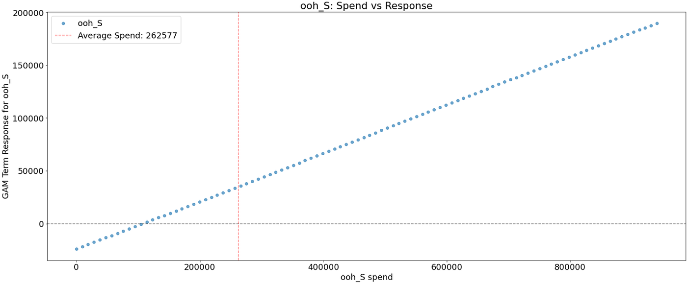
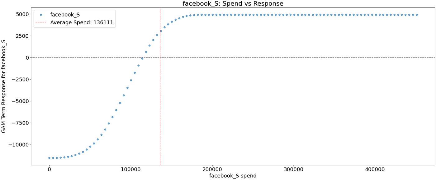
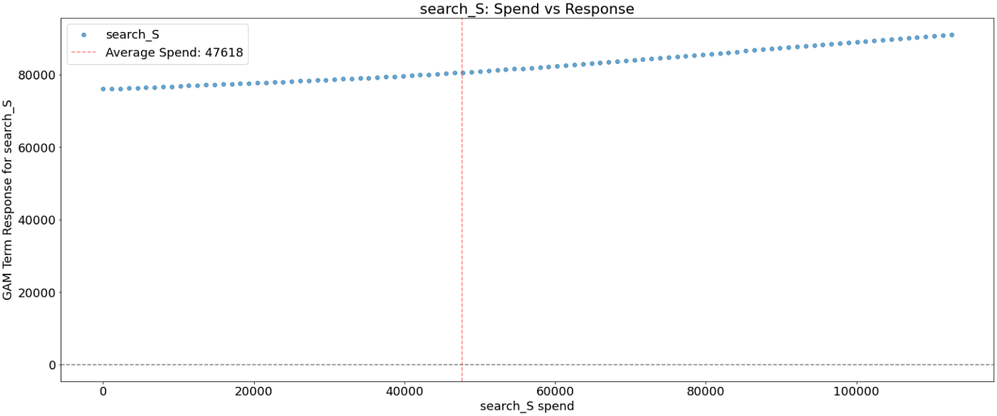
As was anticipated after reviewing the ultimate mannequin, a number of media channels (search_S, ooh_S) have a linear impact.

Taking facebook_S, we observe a powerful s-shape of the diminishing returns that implies that commercial spend beginning near 200K gained’t deliver any further enhance within the response.

Taking print_S, its response fee declines at about 125K spend

Observing search_S, its response fee will increase nearly linearly however at a really gradual fee.

On this article, I confirmed one more method for modeling advertising and marketing combine by making use of penalized smoothing splines on media channels. This method doesn’t require reworking media spend variables to account for non-linearities of diminishing returns. Lastly, smoothing splines resulted in a greater mannequin match in comparison with the linear regression fashions, which will increase confidence within the decomposed results.

The whole code may be downloaded from my Github repo

Thanks for studying!