Lung Most cancers Detection utilizing Convolutional Neural Community (CNN)

Pc Imaginative and prescient is without doubt one of the functions of deep neural networks that permits us to automate duties that earlier required years of experience and one such use in predicting the presence of cancerous cells.

On this article, we’ll discover ways to construct a classifier utilizing a easy Convolution Neural Community which may classify regular lung tissues from cancerous. This undertaking has been developed utilizing collab and the dataset has been taken from Kaggle whose hyperlink has been offered as effectively.

The method which will likely be adopted to construct this classifier:

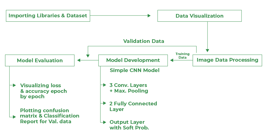
Circulate Chart for the Challenge

Modules Used

Python libraries make it very simple for us to deal with the information and carry out typical and sophisticated duties with a single line of code.

• Pandas – This library helps to load the information body in a 2D array format and has a number of capabilities to carry out evaluation duties in a single go.
• Numpy – Numpy arrays are very quick and may carry out massive computations in a really quick time.
• Matplotlib – This library is used to attract visualizations.
• Sklearn – This module comprises a number of libraries having pre-implemented capabilities to carry out duties from knowledge preprocessing to mannequin improvement and analysis.
• OpenCV – That is an open-source library primarily centered on picture processing and dealing with.
• Tensorflow – That is an open-source library that’s used for Machine Studying and Synthetic intelligence and gives a spread of capabilities to attain advanced functionalities with single traces of code.

Importing Dataset

The dataset which we’ll use right here has been taken from -https://www.kaggle.com/datasets/andrewmvd/lung-and-colon-cancer-histopathological-images.  This dataset consists of 5000 photographs for 3 courses of lung circumstances:

• Regular Class
• Lung Adenocarcinomas
• Lung Squamous Cell Carcinomas

These photographs for every class have been developed from 250 photographs by performing Knowledge Augmentation on them. That’s the reason we gained’t be utilizing Knowledge Augmentation additional on these photographs.

Output:

The information set has been extracted.

Knowledge Visualization

On this part, we’ll attempt to perceive visualize some photographs which have been offered to us to construct the classifier for every class.

Output:

['lung_n', 'lung_aca', 'lung_scc']

These are the three courses that we’ve right here.

Output:

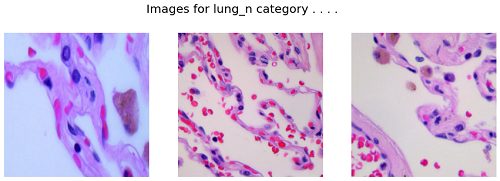
Photographs for lung_n class

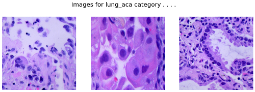
Photographs for lung_aca class

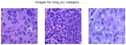
Photographs for lung_scc class

The above output could fluctuate if you’ll run this in your pocket book as a result of the code has been applied in such a manner that it’s going to present completely different photographs each time you rerun the code.

Knowledge Preparation for Coaching

On this part, we’ll convert the given photographs into NumPy arrays of their pixels after resizing them as a result of coaching a Deep Neural Community on large-size photographs is extremely inefficient by way of computational value and time.

For this goal, we’ll use the OpenCV library and Numpy library of python to serve the aim. Additionally, in spite of everything the photographs are transformed into the specified format we’ll break up them into coaching and validation knowledge so, that we are able to consider the efficiency of our mannequin.

Among the hyperparameters which we are able to tweak from right here for the entire pocket book.

One scorching encoding will assist us to coach a mannequin which may predict smooth possibilities of a picture being from every class with the best likelihood for the category to which it actually belongs.

Output:

(12000, 256, 256, 3) (3000, 256, 256, 3)

On this step, we’ll obtain the shuffling of the information robotically as a result of the train_test_split operate break up the information randomly within the given ratio.

Mannequin Improvement

From this step onward we’ll use the TensorFlow library to construct our CNN mannequin. Keras framework of the tensor move library comprises all of the functionalities that one could have to outline the structure of a Convolutional Neural Community and prepare it on the information.

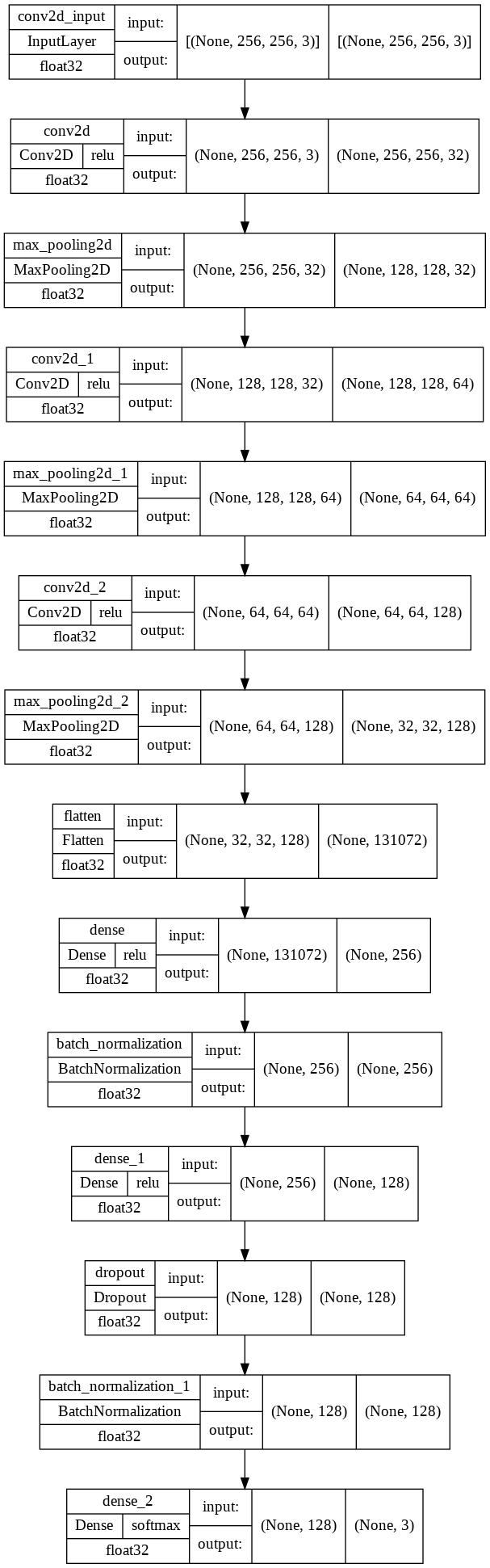
Mannequin Structure

We’ll implement a Sequential mannequin which can include the next components:

• Three Convolutional Layers adopted by MaxPooling Layers.
• The Flatten layer to flatten the output of the convolutional layer.
• Then we can have two totally related layers adopted by the output of the flattened layer.
• We’ve got included some BatchNormalization layers to allow secure and quick coaching and a Dropout layer earlier than the ultimate layer to keep away from any chance of overfitting.
• The ultimate layer is the output layer which outputs smooth possibilities for the three courses. 

Let’s print the abstract of the mannequin’s structure:

Output:

Mannequin: “sequential”

_________________________________________________________________

 Layer (sort)                Output Form              Param #   

=================================================================

 conv2d (Conv2D)             (None, 256, 256, 32)      2432      

                                                                 

 max_pooling2d (MaxPooling2D  (None, 128, 128, 32)     0         

 )                                                               

                                                                 

 conv2d_1 (Conv2D)           (None, 128, 128, 64)      18496     

                                                                 

 max_pooling2d_1 (MaxPooling  (None, 64, 64, 64)       0         

 2D)                                                             

                                                                 

 conv2d_2 (Conv2D)           (None, 64, 64, 128)       73856     

                                                                 

 max_pooling2d_2 (MaxPooling  (None, 32, 32, 128)      0         

 2D)                                                             

                                                                 

 flatten (Flatten)           (None, 131072)            0         

                                                                 

 dense (Dense)               (None, 256)               33554688  

                                                                 

 batch_normalization (BatchN  (None, 256)              1024      

 ormalization)                                                   

                                                                 

 dense_1 (Dense)             (None, 128)               32896     

                                                                 

 dropout (Dropout)           (None, 128)               0         

                                                                 

 batch_normalization_1 (Batc  (None, 128)              512       

 hNormalization)                                                 

                                                                 

 dense_2 (Dense)             (None, 3)                 387       

                                                                 

=================================================================

Complete params: 33,684,291

Trainable params: 33,683,523

Non-trainable params: 768

_________________________________________________________________

From above we are able to see the change within the form of the enter picture after passing via completely different layers. The CNN mannequin we’ve developed comprises about 33.5 Million parameters. This large variety of parameters and complexity of the mannequin is what helps to attain a high-performance mannequin which is being utilized in real-life functions.

Output:

Modifications within the form of the enter picture.

Whereas compiling a mannequin we offer these three important parameters:

• optimizer – That is the tactic that helps to optimize the associated fee operate through the use of gradient descent.
• loss – The loss operate by which we monitor whether or not the mannequin is bettering with coaching or not.
• metrics – This helps to judge the mannequin by predicting the coaching and the validation knowledge.

Callback

Callbacks are used to verify whether or not the mannequin is bettering with every epoch or not. If not then what are the required steps to be taken like ReduceLROnPlateau decreases studying price additional. Even then if mannequin efficiency isn’t bettering then coaching will likely be stopped by EarlyStopping. We will additionally outline some customized callbacks to cease coaching in between if the specified outcomes have been obtained early.

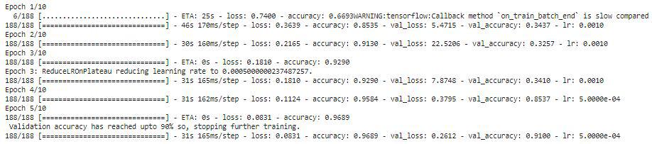
Now we’ll prepare our mannequin:

Output:

 

Let’s visualize the coaching and validation accuracy with every epoch.

Output:

 

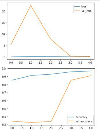
From the above graphs, we are able to definitely say that the mannequin has not overfitted the coaching knowledge because the distinction between the coaching and validation accuracy may be very low.

Mannequin Analysis

Now as we’ve our mannequin prepared let’s consider its efficiency on the validation knowledge utilizing completely different metrics. For this goal, we’ll first predict the category for the validation knowledge utilizing this mannequin after which examine the output with the true labels.

Let’s draw the confusion metrics and classification report utilizing the expected labels and the true labels.

Output:

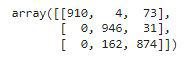
Confusion Matrix for the validation knowledge.

Output:

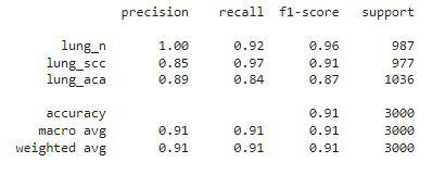
Classification Report for the Validation Knowledge

Conclusion:

Certainly the efficiency of our easy CNN mannequin is excellent because the f1-score for every class is above 0.90 which implies our mannequin’s prediction is appropriate 90% of the time. That is what we’ve achieved with a easy CNN mannequin what if we use the Switch Studying Method to leverage the pre-trained parameters which have been educated on tens of millions of datasets and for weeks utilizing a number of GPUs? It’s extremely more likely to obtain even higher efficiency on this dataset.