Home Value Prediction utilizing Machine Studying in Python

September 5, 2022

2

All of us have skilled a time when we’ve got to lookup for a brand new home to purchase. However then the journey begins with plenty of frauds, negotiating offers, researching the native areas and so forth.

Home Value Prediction utilizing Machine Studying

So to cope with this sort of points Immediately we might be getting ready a MACHINE LEARNING Based mostly mannequin, educated on the Home Value Prediction Dataset.

You’ll be able to obtain the dataset from this hyperlink.

The dataset accommodates 13 options :

1	Id	To rely the information.
2	MSSubClass	Identifies the kind of dwelling concerned within the sale.
3	MSZoning	Identifies the final zoning classification of the sale.
4	LotArea	Lot dimension in sq. ft.
5	LotConfig	Configuration of the lot
6	BldgType	Kind of dwelling
7	OverallCond	Charges the general situation of the home
8	YearBuilt	Unique building 12 months
9	YearRemodAdd	Transform date (similar as building date if no reworking or additions).
10	Exterior1st	Exterior masking on home
11	BsmtFinSF2	Kind 2 completed sq. ft.
12	TotalBsmtSF	Complete sq. ft of basement space
13	SalePrice	To be predicted

Importing Libraries and Dataset

Right here we’re utilizing

Pandas – To load the Dataframe
Matplotlib – To visualise the info options i.e. barplot
Seaborn – To see the correlation between options utilizing heatmap

Python3

import pandas as pd

import matplotlib.pyplot as plt

import seaborn as sns

dataset = pd.read_excel("HousePricePrediction.xlsx")

print(dataset.head(5))

Output:

As we’ve got imported the info. So form technique will present us the dimension of the dataset.

Output:

(2919,13)

Knowledge Preprocessing

Now, we categorize the options relying on their datatype (int, float, object) after which calculate the variety of them.

Python3

obj = (dataset.dtypes == 'object')

object_cols = record(obj[obj].index)

print("Categorical variables:",len(object_cols))

int_ = (dataset.dtypes == 'int')

num_cols = record(int_[int_].index)

print("Integer variables:",len(num_cols))

fl = (dataset.dtypes == 'float')

fl_cols = record(fl[fl].index)

print("Float variables:",len(fl_cols))

Output:

Categorical variables : 4
Integer variables : 6
Float varibales : 3

Exploratory Knowledge Evaluation

EDA refers back to the deep evaluation of information in order to find totally different patterns and spot anomalies. Earlier than making inferences from knowledge it’s important to look at all of your variables.

So right here let’s make a heatmap utilizing seaborn library.

Python3

plt.determine(figsize=(12, 6))

sns.heatmap(dataset.corr(),

cmap = 'BrBG',

fmt = '.2f',

linewidths = 2,

annot = True)

Output:

To research the totally different categorical options. Let’s draw the barplot.

Python3

unique_values = []

for col in object_cols:

unique_values.append(dataset[col].distinctive().dimension)

plt.determine(figsize=(10,6))

plt.title('No. Distinctive values of Categorical Options')

plt.xticks(rotation=90)

sns.barplot(x=object_cols,y=unique_values)

Output:

The plot reveals that Exterior1st has round 16 distinctive classes and different options have round 6 distinctive classes. To findout the precise rely of every class we are able to plot the bargraph of every 4 options individually.

Python3

plt.determine(figsize=(18, 36))

plt.title('Categorical Options: Distribution')

plt.xticks(rotation=90)

index = 1

for col in object_cols:

y = dataset[col].value_counts()

plt.subplot(11, 4, index)

plt.xticks(rotation=90)

sns.barplot(x=record(y.index), y=y)

index += 1

Output:

Knowledge Cleansing

Knowledge Cleansing is the best way to improvise the info or take away incorrect, corrupted or irrelevant knowledge.

As in our dataset, there are some columns that aren’t necessary and irrelevant for the mannequin coaching. So, we are able to drop that column earlier than coaching. There are 2 approaches to coping with empty/null values

We will simply delete the column/row (if the characteristic or report will not be a lot necessary).
Filling the empty slots with imply/mode/0/NA/and many others. (relying on the dataset requirement).

As Id Column won’t be taking part in any prediction. So we are able to Drop it.

Python3

dataset.drop(['Id'],

axis=1,

inplace=True)

Changing SalePrice empty values with their imply values to make the info distribution symmetric.

Python3

dataset['SalePrice'] = dataset['SalePrice'].fillna(

dataset['SalePrice'].imply())

Drop information with null values (because the empty information are very much less).

Python3

new_dataset = dataset.dropna()

Checking options which have null values within the new dataframe (if there are nonetheless any).

Python3

new_dataset.isnull().sum()

Output:

OneHotEncoder – For Label categorical options

One scorching Encoding is the easiest way to transform categorical knowledge into binary vectors. This maps the values to integer values. By utilizing OneHotEncoder, we are able to simply convert object knowledge into int. So for that, firstly we’ve got to gather all of the options which have the item datatype. To take action, we’ll make a loop.

Python3

from sklearn.preprocessing import OneHotEncoder

s = (new_dataset.dtypes == 'object')

object_cols = record(s[s].index)

print("Categorical variables:")

print(object_cols)

print('No. of. categorical options: ',

len(object_cols))

Output:

Then as soon as we’ve got an inventory of all of the options. We will apply OneHotEncoding to the entire record.

Python3

OH_encoder = OneHotEncoder(sparse=False)

OH_cols = pd.DataFrame(OH_encoder.fit_transform(new_dataset[object_cols]))

OH_cols.index = new_dataset.index

OH_cols.columns = OH_encoder.get_feature_names()

df_final = new_dataset.drop(object_cols, axis=1)

df_final = pd.concat([df_final, OH_cols], axis=1)

Splitting Dataset into Coaching and Testing

X and Y splitting (i.e. Y is the SalePrice column and the remainder of the opposite columns are X)

Python3

from sklearn.metrics import mean_absolute_error

from sklearn.model_selection import train_test_split

X = df_final.drop(['SalePrice'], axis=1)

Y = df_final['SalePrice']

X_train, X_valid, Y_train, Y_valid = train_test_split(

X, Y, train_size=0.8, test_size=0.2, random_state=0)

Mannequin and Accuracy

As we’ve got to coach the mannequin to find out the continual values, so we might be utilizing these regression fashions.

SVM-Help Vector Machine
Random Forest Regressor
Linear Regressor

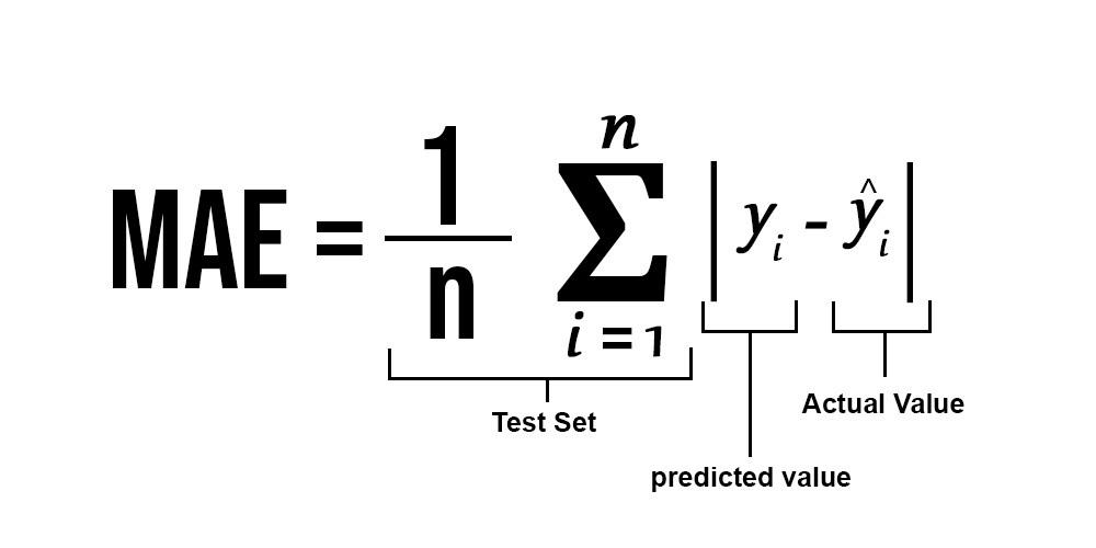
And To calculate loss we might be utilizing the mean_absolute_percentage_error module. It could simply be imported through the use of sklearn library. The method for Imply Absolute Error :

SVM – Help vector Machine

SVM can be utilized for each regression and classification mannequin. It finds the hyperplane within the n-dimensional aircraft. To learn extra about svm refer this.

Python3

from sklearn import svm

from sklearn.svm import SVC

from sklearn.metrics import mean_absolute_percentage_error

model_SVR = svm.SVR()

model_SVR.match(X_train,Y_train)

Y_pred = model_SVR.predict(X_valid)

print(mean_absolute_percentage_error(Y_valid, Y_pred))

Output :

0.18705129

Random Forest Regression

Random Forest is an ensemble approach that makes use of a number of of determination timber and can be utilized for each regression and classification duties. To learn extra about random forests refer this.

Python3

from sklearn.ensemble import RandomForestRegressor

model_RFR = RandomForestRegressor(n_estimators=10)

model_RFR.match(X_train, Y_train)

Y_pred = model_RFR.predict(X_valid)

mean_absolute_percentage_error(Y_valid, Y_pred)

Output :

0.1929469

Linear Regression

Linear Regression predicts the ultimate output-dependent worth primarily based on the given impartial options. Like, right here we’ve got to foretell SalePrice relying on options like MSSubClass, YearBuilt, BldgType, Exterior1st and many others. To learn extra about Linear Regression refer this.

Python3

from sklearn.linear_model import LinearRegression

model_LR = LinearRegression()

model_LR.match(X_train, Y_train)

Y_pred = model_LR.predict(X_valid)

print(mean_absolute_percentage_error(Y_valid, Y_pred))

Output :

0.187416838

Conclusion

Clearly, SVM mannequin is giving higher accuracy because the imply absolute error is the least amongst all the opposite regressor fashions i.e. 0.18 approx. To get a lot better outcomes ensemble studying methods like Bagging and Boosting will also be used.

Previous articleUnit testing with React and Cypress

Next articleFinest practices to publish open-source software program operators

Home Value Prediction utilizing Machine Studying in Python

Home Value Prediction utilizing Machine Studying

Importing Libraries and Dataset

Python3

Knowledge Preprocessing

Python3

Exploratory Knowledge Evaluation

Python3

Python3

Python3

Knowledge Cleansing

Python3

Python3

Python3

Python3

OneHotEncoder – For Label categorical options

Python3

Python3

Splitting Dataset into Coaching and Testing

Python3

Mannequin and Accuracy

SVM – Help vector Machine

Python3

Random Forest Regression

Python3

Linear Regression

Python3

Conclusion

LEAVE A REPLY Cancel reply

Most Popular

Recent Comments

ABOUT US

POPULAR POSTS

POPULAR CATEGORY