Learn to visualize textual content knowledge to convey your story
There are numerous definitions of Pure Language Processing (NLP) however the one I usually quote is the next:
NLP strives to construct machines that perceive and reply to textual content or voice knowledge — and reply with textual content or speech of their very own — in a lot the identical method people do. [1]
The NLP market is rising quick due to the rising quantities of textual content knowledge which might be being generated in quite a few purposes, platforms and businesses. Thus, it’s essential to realizing find out how to convey significant and fascinating tales from textual content knowledge. For that, you want visualization. On this publish, allow us to be taught on find out how to get began on visualizing textual content knowledge. Extra superior strategies of pre-processing and visualizing textual content knowledge will likely be launched in one other publish!
The idea of “abstract statistics” for tabular knowledge applies to textual content knowledge similarly. Abstract statistics assist us characterize knowledge. Within the context of textual content knowledge, such statistics could be issues like variety of phrases that make up every textual content and the way the distribution of that statistic appears to be like like throughout your complete corpus. For distributions, we will use visualizations together with the kernel density estimate (KDE) plot and histogram and so on. however for the aim of simply introducing what statistic might be thought of for visualization, the .hist( ) operate is utilized in all of the code snippets.
Say we’ve a overview dataset which comprises a variable named “description” with textual content descriptions in it.
[1] size of every textual content
critiques[‘description’].str.len().hist()
[2] Phrase depend in every textual content
# .str.cut up( ) returns an inventory of phrases cut up by the required delimiter
# .map(lambda x: len(x)) utilized on .str.cut up( ) will return the variety of cut up phrases in every textual contentcritiques[‘description’].str.cut up().map(lambda x: len(x)).hist()
One other option to do it:
critiques[‘description’].apply(lambda x: len(str(x).cut up())).hist()
[3] Distinctive phrase depend in every textual content
critiques[‘description’].apply(lambda x: len(set(str(x).cut up()))).hist()
[4] Imply phrase size in every textual content
critiques[‘description’].str.cut up().apply(lambda x : [len(i) for i in x]).map(lambda x: np.imply(x)).hist()
One other option to do it:
critiques[‘description’].apply(lambda x: np.imply([len(w) for w in str(x).split()])).hist()
[5] Median phrase size in every textual content (Distribution)
critiques[‘description’].apply(lambda x: np.median([len(w) for w in str(x).split()])).hist()
[6] Cease phrase depend
Stopwords within the NLP context refers to a set of phrases that often seem within the corpus however don’t add a lot that means to understanding varied points of the textual content together with sentiment and polarity. Examples are pronouns (e.g. he, she) and articles (e.g. the).
There are primarily two methods to retrieve stopwords. A technique is to make use of the NLTK bundle and the opposite is to make use of the wordcloud bundle as an alternative. Right here, I take advantage of the wordcloud bundle because it already has a full set of English stopwords predefined in a sub-module referred to as “STOPWORDS”.
from wordcloud import STOPWORDS### Different option to retrieve stopwords# import nltk# nltk.obtain(‘stopwords’)# stopwords =set(stopwords.phrases(‘english’))
critiques[‘description’].apply(lambda x: len([w for w in str(x).lower().split() if w in STOPWORDS])).hist()
[7] Character Rely
critiques[‘description’].apply(lambda x: len(str(x))).hist()
[8] Punctuation Rely
critiques[‘description’].apply(lambda x: len([c for c in str(x) if c in string.punctuation])).hist()
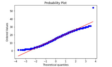
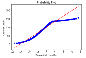
Bonus: Checking Normality
For brand new statistic variables (e.g. imply phrase size) created, you could need to c heck whether or not they meet sure situations as sure fashions or regression algorithms require variables to fall underneath sure distributions, for instance. One such test could be checking if the distribution of a variable is shut sufficient to a traditional distribution by trying on the likelihood plot.
from scipy import stats
import statsmodels.api as smstats.probplot(critiques['char_length'], plot=plt)
What’s an n-gram? In response to Stanford’s Speech and Language Processing class materials, an “n-gram is a sequence n-gram of n phrases in a sentence of textual content.” [2]
As an illustration, bigrams (n-gram with n=2) of the sentence “I’m cool” could be:
[ (‘I’, ‘am”), (‘am’, ‘cool’)]
To visualise probably the most often showing high N-Grams, we have to first signify our vocabulary into some numeric matrix type. To do that, we use the Countvectorizer. In response to Python’s scikit-learn bundle documentation, “Countvectorizer is a technique that converts a set of textual content paperwork to a matrix of token counts.” [3]
The next operate first vectorizes textual content into some acceptable matrix type that comprises the counts of tokens (right here n-grams). Observe that the argument stop_words might be specified to omit the stopwords from the required language when doing the counts.
def ngrams_top(corpus, ngram_range, n=None): ### What this operate does: Record the highest n phrases in a vocabulary in keeping with incidence in a textual content corpus. vec = CountVectorizer(stop_words = ‘english’, ngram_range=ngram_range).match(corpus) bag_of_words = vec.rework(corpus) sum_words = bag_of_words.sum(axis=0) words_freq = [(word, sum_words[0, idx]) for phrase, idx in vec.vocabulary_.gadgets()] words_freq =sorted(words_freq, key = lambda x: x[1], reverse=True) total_list=words_freq[:n] df = pd.DataFrame(total_list, columns=[‘text’,’count’]) return df
The next operate specified the ngram_range to be (1,1), so we’re solely all in favour of unigrams that are principally simply particular person phrases. n=10 right here means we’re all in favour of trying on the high 10 unigrams within the corpus of descriptions.
unigram_df = ngrams_top(critiques[‘description’], (1,1), n=10)
We then can visualize this right into a horizontal bar plot utilizing seaborn.
# seaborn barplotsns.barplot(x=’depend’, y=’textual content’) #horizontal barplot
If you wish to use a barely fancier and interactive type of visualization, I like to recommend plotly specific which has quite simple syntax however lets you create interactive visualizations in just a few strains of code.
# fancier interactive plot utilizing plotly specificimport plotly.specific as pxfig = px.bar(unigram_df, x='unigram', y='depend', title=’Counts of high unigrams', template='plotly_white', labels={'ngram;: ‘Unigram’, ‘depend’: ‘Rely’})fig.present()
Extra superior strategies of pre-processing and visualizing textual content knowledge will likely be launched in one other publish!
Knowledge Scientist. Incoming PhD pupil in Informatics at UC Irvine.
Former analysis space specialist on the Legal Justice Administrative Information System (CJARS) economics lab on the College of Michigan, engaged on statistical report era, automated knowledge high quality overview, constructing knowledge pipelines and knowledge standardization & harmonization. Former Knowledge Science Intern at Spotify. Inc. (NYC).
He loves sports activities, working-out, cooking good Asian meals, watching kdramas and making / performing music and most significantly worshiping Jesus Christ, our Lord. Checkout his web site!
[1] What’s Pure Language Processing?, IBM Cloud, https://realpython.com/python-assert-statement/
[2] D. Jurafsky & J. H. Martin. Speech and Language Processing (Final Up to date December, 2021). https://internet.stanford.edu/~jurafsky/slp3/3.pdf
[3] Scikit Study documentation. https://scikit-learn.org/secure/modules/generated/sklearn.feature_extraction.textual content.CountVectorizer.html
