Exploring larger dimensional objects with laptop science algorithms
The applicability of graph concept within the context of web2.0 is apparent, with web sites like Fb (undirected graph of friendships) and Twitter (directed graph of followings) constructed round them. One other apparent utility is in laptop networks. The sector of operations analysis, which began with making use of math to the sector of battlefield logistics is chock stuffed with graph concept issues as effectively. For example, see right here.
However graph concept is so versatile, it finds functions in information science as effectively. Other than the truth that neural networks are particular sorts of graphs, it’s entrance and middle within the area of combinatorial testing, the place we design experiments in a means that necessary properties or mixtures of properties are lined. For example, see right here. That is the context through which I first began studying about it.
On this article, we’ll be overlaying a unique utility nonetheless. Since I used to be a toddler, I used to be fascinated with the 4 dimensional dice. I needed to carry it in my hand and manipulate it like I can with a 3-D dice. Little did I do know that the lacking piece was graph concept (a software I added to my arsenal solely lately on account of its functions in information science), as we’ll see.
I-A) Flattening a dice
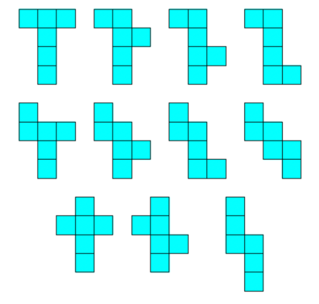
A dice is an object that lives in third-dimensional house and is acquainted to most (suppose bins). It has six equivalent sq. faces and 12 edges between a few of these faces. What do you do with cubical bins? You narrow them open (to see what’s inside). That is usually performed by reducing alongside the perimeters. There are methods to do that such that the six faces nonetheless keep linked to the principle physique and lie flat on the ground. It turns on the market are 11 topologically distinct (which means you may’t translate and rotate one and make it completely overlap with some other) meshes that emerge after we make the cuts in numerous methods. These are proven under.

Discover that in every of the meshes, there are precisely 5 surviving edges. This isn’t a coincidence. If we consider the faces of the dice because the vertices of a graph and the surviving edges as the perimeters of that graph, then every of the meshes within the determine above is a spanning tree. Which implies that there’s precisely one path that connects any two vertices. Since there have been twelve edges within the unique dice, we reduce precisely seven of them to get any of the eleven meshes. The overall variety of methods of choosing the seven edges to chop is {12 select 7} = 792. However a whole lot of these don’t result in spanning bushes since one or two of the faces are fully remoted from the remainder of the physique. It seems that barely lower than half of these cuts result in spanning bushes, 384. And each spanning tree results in a sound mesh. Amongst these 384 meshes, most are repetitions of beforehand seen ones if we rotate and translate them (which means they’re topologically equal). In different phrases, if we will place one mesh on one other in any means such that the latter fully covers the previous, these two are thought of the identical mesh. So solely 11 topologically distinct ones pictured above emerge.
It’s unclear when some human first counted out these 11 meshes. It’s a drawback that may be solved in an affordable period of time with out a pc. So whether or not or not it was thought of and solved earlier than the arrival of computer systems is an fascinating query. Most authors at this time reference [1] from 1984. In [2], Gardner poses the query on what number of meshes exist and it seems he knew the reply (in 1966), although he doesn’t state it explicitly.
For those who’re questioning about functions of this sort of factor, BTW, one instance is photo voltaic sails which should be compact whereas launching and unfold into one thing with a big floor space.
I-B) Flattening a Tesseract
The idea of a dice exists may be prolonged to house of any dimensionality. In two dimensions, we have now the sq.. And in 4 dimensions, we get a Tesseract, a 4 dimensional object composed of three dimensional cubes. Similar to a 3-D dice may be flattened into 2-d house to type a mesh of squares, so can a Tesseract be flattened into 3-D house to type a mesh of 3-D cubes.
The query on what number of such meshes exist was posed in 1966 by Gardner (see web page x of [2]). Answered in 1985 (261 meshes) in [1] by way of a brand new idea known as “paired bushes”. The meshes have been lastly visualized in 2015 within the MathOverflow put up, [3].
What nobody appears to have thought of to this point is flattening a 4-d dice all the way in which to 2-d house right into a mesh of squares. That is what we’ll discover in part III. However first, let’s describe some notation.
On this part, we set up some notation for figuring out the varied parts of an n-dimensional dice. Let’s begin with a 2-d dice or a sq.. We place it in a means that the middle of the sq. is on the origin, (0,0) as proven in determine 2 under.

For brevity, we name your complete sq. “00” as a result of its middle of mass occurs to lie at (0,0). The middle of the highest fringe of the sq. is (0,+1). Once more, for the sake of brevity, we title it simply “0+”. Equally, the underside edge is known as 0-. The left edge is “-0” and the best one is “+0”. The highest left vertex is (-1,+1) and so we name it “-+” and so forth.
For any given entity of the dice in d-dimensional house, its title is represented by d characters, every of which may be one in every of -, 0 or +. A string of all zeros is the middle of the dice (and there is just one). One of many zeros changed by both a + or a — turns into a set of (d-1) dimensional cubes. There are 2*d such cubes (d methods of selecting the place the non-zero character will lie after which assigning it both a + or a -). Equally, there are d*(d-1)/2*4 = 2*d*(d-1) cubes of dimension (d-2) (select two areas that for the non-zero characters after which fill then each with “+” or “-” in 4 methods) and so forth.
We noticed in part (I) the way it was potential to flatten a 3-D dice to a 2-d desk such that each one the faces stayed linked and none of them overlapped. Is it potential to do the identical factor with a 4-d dice or Tesseract? Considerably surprisingly, the reply is sure. Proven under is one such mesh. I obtained it by fastidiously flattening out simply the “high” 3-D dice to a desk with a few of the faces nonetheless connected, after which making an attempt to flatten the remaining faces by hit and trial in a means that they wouldn’t overlap.

The plain query is, what number of such meshes exist?
III-A) Properties of legitimate meshes
For the legitimate meshes of a dice from figure-1, we word two key properties that additionally maintain for the mesh of a Tesseract in figure-2:
- It’s clear that each one the faces are nonetheless linked to one another (by definition). So, it’s potential to begin at any of the faces within the mesh and attain some other.
- Additionally word that between any two faces, there’s at most one edge. This was true of the unique Dice or Tesseract, so it should be true of the mesh as effectively.
Combining the above two details and pondering of the faces of the stable as vertices of a graph, it’s clear that the mesh kinds a spanning tree (a graph with all vertices reachable from any vertex and at most one edge between any two vertices). This perception was most likely step one utilized by Turney in [1] to rely the 3-D meshes of a Tesseract. So, each legitimate 2-d mesh of a dice or Tesseract (or for that matter, any (d<n) dimensional mesh of an n-dimensional dice) is a sound spanning tree if the faces are thought of vertices of a graph. One property of a spanning tree with n vertices is that it has precisely n-1 edges. Let’s visualize this graph of the faces of the Tesseract from which the spanning bushes that then grow to be the meshes are constructed.

For the case of the dice, every bodily edge maps 1:1 with a graph edge (this may appear apparent, however you’ll see later why I known as it out). So, we begin with 12 edges and have to chop precisely 7 edges (so 6–1=5 stay) earlier than “opening it up” right into a mesh (which is why all of the meshes in determine 1 had 5 edges linked). As soon as we make the 7 cuts (in a means that each one the vertices stay reachable from one another), there is just one option to flatten to a mesh.
For a Tesseract, every bodily edge really corresponds to a few edges of the graph. It is because three faces meet at each bodily edge (versus 2 for a dice). So whereas the variety of bodily edges is simply 32, the variety of graph edges (within the graph the place every face is a vertex) is definitely 32*3 = 96 (3 methods to decide on 2 of the faces assembly at every bodily edge). Of those 96 graph edges, solely 23 can stay within the flattened mesh. For a given bodily edge, if all three graph edges are intact, it is going to be unimaginable to flatten the Tesseract to a desk with out overlap.
IV-A) The essential operation
Let’s say we have now a spanning tree of the Tesseract face graph that may be flattened right into a mesh, expressed as an adjacency checklist. How will we go from this graph to the precise flattened Tesseract mesh (like figure-2)? We are able to think about doing this by rotating the faces as we might within the bodily world. Any two linked faces of the d-dimensional dice are perpendicular. For instance, two faces (per nomenclature in part II) 00- and -00 of the 3-D dice. Notice that within the figures of this part, I’ve shifted the origin from the middle of the dice to one of many vertices to make the flattening course of clearer.

We are able to at all times repair one of many faces and rotate the opposite one to its aircraft alongside the sting connecting them as proven within the determine above. That is the essential operation we’ll construct on high of. Notice that irrespective of how massive the dimensionality of the house this unfolding occurs in, the preliminary and ultimate configurations are distinctive. There’s at all times a easy rotation concerning the frequent edge becoming a member of the 2 faces (right here, the y-axis) which may be expressed in matrix type. Within the instance above, this rotation matrix (rotation within the x-z aircraft) is:

One subtlety when performing this on a pc is that the rotation (relying on climate the angle is constructive or unfavorable) might deliver the -00 face on high of or adjoining to the 00- face. We wish to keep away from the rotation that makes the faces overlap. If plugging in pi/2 into the rotation matrix causes the faces to overlap, we merely plug in -pi/2.
IV-B) Two easy meshes
Now, let’s take simply three faces of a 3-D dice. Say 00-, 0–0 and -00. These three faces are proven within the determine under.

Within the unique dice, they’re all linked to one another. The face graph of those three faces would appear to be the determine 7-a.

However this isn’t a tree. In a tree, there is just one path between any two vertices. Within the graph above, there are two paths between -00 and 0–0 (direct and by way of the third vertex, 00-). To make it a tree, we have now to chop off one of many edges. In determine 3-b we select to chop the highest edge between -00 and 0–0. Now that we have now a tree, we have to get the corresponding mesh.
First, we choose the face whose aircraft all different faces are going to rotate into within the flattened mesh. If we have been opening up a cubical field, this may be the face that rests on the ground. This one is the “base face” and the selection is bigoted. Within the instance above, we select 00- (the underside face within the determine) as the bottom face.
Right here, the remaining two faces are linked on to the bottom face. We are able to merely rotate each of them right down to the aircraft of the bottom face independently, as within the “primary operation” described earlier, acquiring the mesh under.

This was a straightforward instance, with each faces we needed to rotate straight linked to the bottom face. Let’s return to determine 7-a and this time reduce the sting between 0–0 and 00-. We get one other legitimate spanning tree. And let’s maintain the bottom face the identical, 00-.

Now, we have now to do the rotations in two steps. The 0–0 face is linked to the -00 face. If we rotate the -00 face first, the rotation required to deliver the 0–0 face to its aircraft (the rotation matrix in addition to axis about which to rotate) will change (since every part would have rotated now). To keep away from this, we rotate the 0–0 face and produce it into the aircraft of -00 first. Solely then will we deliver each these faces to the x-y aircraft the place the 00- face lies. This sequence of operations is demonstrated under.

Notice that right here, the 0–0 face wanted two rotations because it was two hops from the bottom face (00-) within the tree whereas the -00 face wanted one rotation because it was one hop from the bottom face. Armed with the instinct from these two circumstances, we will develop a common algorithm for flattening a dice right into a 2-d mesh, given the spanning tree of the perimeters we select to protect.
IV-C) Algorithm for performing the rotations
An algorithm may be devised that applies the rotations to all of the faces in the best order, given the spanning tree to go from the d-dimensional dice to the mesh. First, we all know that each one faces of the dice must be visited (and sure operations should be carried out to the faces in these visits). For the reason that faces are expressed as a graph, a graph exploration algorithm is the very first thing that involves thoughts (algorithms that discover all of the vertices of a graph).
The best and most well-known graph exploration algorithm is named depth first search (DFS; see part 22.3 of Introduction to Algorithms by Cormen et.al., [4]). We apply it not on the unique graph of the Tesseract, however on the spanning tree (which can be a graph, simply with a a lot smaller variety of edges), beginning on the base face. It is because it’s the spanning tree that maps to the mesh we’re after.
The essential operation(s) we have to carry out on all faces are rotations to deliver them to the identical aircraft as the bottom face. As we go from one face to the following (performing DFS), we all know the rotation required to deliver the latter to the identical aircraft as the previous per part IV-A. Since we begin on the base face (b), that’s the solely face that doesn’t get any rotation. The faces straight linked to the bottom face (let’s name them the “first layer of faces”) within the spanning tree get one rotation. These linked to this primary layer of faces (the “second layer”) get two rotations (first to deliver them to the identical aircraft because the respective first layer faces after which to that of the bottom face).
For any given face (say f), there’s a path from the bottom face (b) to it within the tree. Beginning on the base face, b, every new face encountered alongside this path has a corresponding rotation that may be utilized to it to deliver it to the identical aircraft because the earlier face within the path. Every of those rotations gathered alongside the trail should be utilized to the given face, f. We are able to maintain a document of all these rotations by way of the depth first search on the tree. There’s a idea of vertex colours in DFS (once more, check with part 22.3 of Cormen et.al, [4]) that may be white, gray or black. White means the vertex of the graph (or tree) hasn’t even been encountered but (all vertices are white at first of the algorithm). Gray means it’s been visited however all of the vertices downstream from it within the exploration haven’t been processed and black means the algorithm is finished processing the vertex and all its downstream vertices as effectively (as soon as the algorithm completes, all vertices are black). So long as we’re nonetheless traversing a path (haven’t accomplished it), all vertices encountered alongside that path shall be marked gray. And so, we will preserve a listing of rotations to be carried out corresponding to every gray vertex (or face). When a vertex is marked black, we merely take away the corresponding rotation from the checklist.
Nevertheless, the order through which these rotations are utilized to a given face (f) can be necessary as we noticed within the second instance of the mesh with three faces from part IV-B. The given face ought to first be rotated to the aircraft of the face it’s straight linked to, then to the one earlier than it within the path and so forth, reverse order till it’s lastly in the identical aircraft as the bottom face. This ensures that we don’t need to replace the rotations as different rotations occur. The “stack” information construction is ideal for this because it has a “final in first out” property (consider a stack of soiled dishes).
So as a substitute of making use of all of the rotations comparable to the gray vertices as we encounter the faces, we retailer the rotation and the face it’s to be utilized to in a stack. As soon as the depth first search has accomplished exploring all vertices, we really apply the rotations by popping one after the other from the stack the faces and corresponding rotations to be utilized. Beneath is a visible demonstration of this algorithm going from the Tesseract to the mesh by performing the required sequence of rotations.

And right here is a Python implementation of the above algorithm.
Here’s a video the place this algorithm is utilized to the acquainted 3-D dice:
Once we noticed our first 2-d mesh in part III (determine 3), we requested what number of there are. And within the absence of a precise reply, we’d like higher and decrease bounds which can be as tight as potential.
We’ll describe in part VI, a option to generate random meshes beginning with one in every of them. If we then maintain solely the topologically distinct meshes, we’ll construct not solely a library of meshes, but in addition a computational decrease sure, which is the distinct quantity we’ve managed to gather. Any theoretical decrease sure will finally be outdated by the computational one. Thus far, the algorithm (I run it infrequently for 10 minutes and add to the mesh assortment) has managed to gather about 600 distinct meshes (and this rely is at all times growing). The present computational decrease sure on the variety of 2-d meshes of a Tesseract is subsequently 600.
For the higher sure, recall the algorithm in part IV-C which generates a sound mesh from a spanning tree of the face graph every time that is potential (which fairly often isn’t). And even among the many meshes we get this fashion, there shall be variations which can be topologically much like different meshes seen beforehand. So, the variety of spanning bushes ought to be a snug higher sure on the variety of distinct meshes.
Furthermore, since each mesh corresponds to a novel spanning tree (however a spanning tree may not yield a mesh), one option to rely the variety of meshes (whereas constructing a library of them as effectively) is to loop by way of all potential spanning bushes. For each, we verify if a mesh is feasible and if it additionally occurs to be a “topologically novel” one (which means we haven’t seen any earlier than that its topologically much like), we put it aside someplace.
The issue is that the variety of spanning bushes seems to be 10²⁰ (may be obtained by making use of Kirchhoff’s matrix tree theorem to the graph in figure-4). So, even when we take a milli second to course of a single spanning tree, it’ll take greater than the present age of the universe to this point to exhaust all of them. The one factor we get from this line of assault is thus a really beneficiant higher sure on the variety of meshes. There are methods to enhance on this, however we received’t get into them for now, since they nonetheless maintain the higher sure at astronomically excessive numbers.
The algorithm in part IV-C will at all times give us a mesh comparable to a spanning tree if such a mesh is feasible (which regularly isn’t the case). If we have now a option to iterate over spanning bushes, we will generate a mesh the place potential
As talked about within the earlier part, one option to get a decrease sure on the variety of distinct meshes is to easily begin producing them and eliminating those which can be topologically the identical as a mesh seen earlier than. Such an algorithm will maintain “accumulating” meshes, a bit just like the coupon collectors drawback and sustaining a “library” of distinct meshes seen to this point. An issue with this method is that we’ll by no means know for certain if and after we’ve seen all meshes. Once we’re very near producing all meshes, it’ll grow to be tougher and tougher to “gather” any extra. In direction of the tip, virtually each mesh we randomly draw may have been seen earlier than. And so, if we’ve generated a whole lot of meshes with out operating throughout a brand new one, it could possibly be as a result of we’ve merely accomplished our assortment or that a number of are left and it has simply grow to be actually onerous to see a brand new one when drawing randomly.
For now, we select to stay with this downside and easily gather as many meshes as we will. Our algorithm has two elements.
The primary begins with a given mesh and generates one other legitimate random mesh from it, that’s assured to be totally different from the earlier one. That is performed by reducing the sting between two linked faces of the primary mesh. This creates two sub-meshes and likewise two sub-trees (the unique spanning tree has been reduce in two). Then, we discover one other two faces (one from the primary sub-mesh, one from the second) to “paste” the 2 sub-trees collectively and create a brand new spanning tree. For the reason that two “sub-trees” are linked once more, the property of with the ability to go from any face to some other face is re-instated. After which, we will use the algorithm in part IV-C to see if this new tree generates a sound mesh. If it doesn’t, we merely generate a brand new tree and maintain going till we discover one other legitimate mesh. The mesh is saved to disk as a textual content file, which is the adjacency checklist of the corresponding spanning tree.
The second half compares the brand new mesh with all current meshes and removes those which were seen earlier than.
These concepts are applied within the following Python code: https://github.com/ryu577/pyray/blob/grasp/pyray/shapes/twod/tst_sq_mesh.py. The second half is admittedly the computational bottle neck. The extra meshes we gather, the dearer it turns into to match a brand new mesh to all of the earlier ones. As talked about, this two-part algorithm may be run in a loop perpetually till it turns into extraordinarily, extraordinarily onerous to search out new meshes.
The issue of enumerating the 2-d meshes of a 4-d dice has two hallmarks of the most well-liked Math issues. It’s straightforward to clarify and body in a means that just about anybody can perceive it. On the similar time, evidently even our most refined instruments are falling in need of fixing it. At a minimal, we will unleash our computing energy on this drawback and uncover near all of the meshes.
_______________________________________________________
For those who appreciated the story, grow to be a referred member 
https://medium.com/@rohitpandey576/membership
[1] Paper 1984 the place 3-D meshes are mapped to paired bushes (https://unfolding.apperceptual.com).
[2] Martin Gardner’s ebook from 1966 (“The colossal ebook of arithmetic”: https://www.logic-books.data/websites/default/recordsdata/the_colossal_book_of_mathematics.pdf)
[3] MathOverflow put up the place all distinct 3-D meshes are plotted (https://mathoverflow.internet/questions/198722/3d-models-of-the-unfoldings-of-the-hypercube/)
[4] Introduction to algorithms by Cormen et.al.
