
With an instance of Random Forest mannequin

All photos except in any other case famous are by the creator.
In machine studying, more often than not you need a mannequin that’s not solely correct but additionally interpretable. One instance is buyer churn prediction — along with understanding who will churn, it’s equally necessary to grasp which variables are crucial in predicting churn to assist enhance our service and product.
Well-liked machine studying packages corresponding to Scikit-learn provide default calculations of characteristic importances for mannequin interpretation. Nonetheless, oftentimes we are able to’t belief these default calculations. On this article, we’re going to use the well-known Titanic knowledge from Kaggle and a Random Forest mannequin for example:
- Why you want a strong mannequin and permutation significance scores to correctly calculate characteristic importances.
- Why it’s good to perceive the options’ correlation to correctly interpret the characteristic importances.
The apply described on this article may also be generalized to different fashions.
The difficulty with Default Function Significance
We’re going to use an instance to point out the downside with the default impurity-based characteristic importances offered in Scikit-learn for Random Forest. The default characteristic significance is calculated based mostly on the imply lower in impurity (or Gini significance), which measures how efficient every characteristic is at decreasing uncertainty. See this nice article for a extra detailed clarification of the maths behind the characteristic significance calculation.
Let’s obtain the well-known Titanic dataset from Kaggle. The information set has passenger data for 1309 passengers on Titanic and whether or not they survived. Here’s a transient description of the columns included.

First, we load the information and separate it right into a predictor set and a response set. Within the predictor set, we add two random variables random_cat and random_num. Since they’re randomly generated, each of the variables ought to have a really low characteristic significance rating.
Second, we do some easy cleansing and transformation of the information. This isn’t the main target of this text.
Third, we construct a easy random forest mannequin.
RF practice accuracy: 1.000.RF check accuracy: 0.814
The mannequin is barely overfitting on the coaching knowledge however nonetheless has respectable efficiency on the testing set. Let’s use this mannequin for now for example some pitfalls of the default characteristic significance calculation. Let’s check out the default characteristic importances.
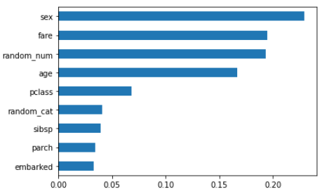
From the default characteristic importances, we discover that:
- The
random_numhas the next significance rating compared withrandom_cat, which confirms that impurity-based importances are biased in the direction of high-cardinality and numerical options. - Non-predictive
random_numvariable is ranked as one of the necessary options, which doesn’t make sense. This displays the default characteristic importances usually are not correct when you have got an overfitting mannequin. When a mannequin overfits, it picks up an excessive amount of noise from the coaching set to make generalized predictions on the check set. When this occurs, the characteristic importances usually are not dependable as they’re calculated based mostly on the coaching set. Extra usually, it solely is smart to have a look at the characteristic importances when you have got a mannequin that may decently predict.
Permutation Significance to Rescue
Then how can we appropriately calculate the characteristic importances? A method is to make use of permutation significance scores. It’s computed with the next steps:
- Practice a baseline mannequin and document the rating (we use accuracy on this instance) on the validation set.
- Re-shuffle values for one characteristic, use the mannequin to foretell once more, and calculate scores on the validation set. The characteristic significance for the characteristic is the distinction between the baseline in 1 and the permutation rating in 2.
- Repeat the method for all options.
Right here we leverage the permutation_importance operate added to the Scikit-learn package deal in 2019. When calling the operate, we set the n_repeats = 20 which implies for every variable, we randomly shuffle 20 instances and calculate the lower in accuracy to create the field plot.
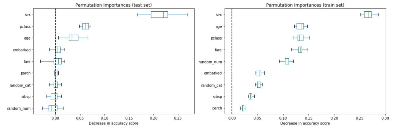
We see that intercourse and pclass present as an important options and random_cat and random_num not have excessive significance scores based mostly on the permutation importances on the check set. The field plot reveals the distribution of the lower in accuracy rating with N repeat permutation (N = 20 in our case).
Let’s additionally compute the permutation importances on the coaching set. This reveals that random_num and random_cat get a considerably greater significance rating than when computed on the check set and the rankings of options look very completely different from the testing set. As famous earlier than, it’s because of the overfitting of the mannequin.
You might surprise why Scikit-learn nonetheless contains the default characteristic significance given it’s not correct. Breiman and Cutler, the inventors of RFs, indicated that this methodology of “including up the Gini decreases for every variable over all bushes within the forest provides a quick variable significance that’s typically very in line with the permutation significance measure.” So the default is supposed to be a proxy for permutation importances. Nonetheless, as Strobl et al identified in Bias in random forest variable significance measures that “the variable significance measures of Breiman’s authentic Random Forest methodology … usually are not dependable in conditions the place potential predictor variables differ of their scale of measurement or their variety of classes.”
A Strong Mannequin is a Prerequisite for Correct Significance Scores
We’ve seen when a mode is overfitting, the characteristic importances generated from the coaching and prediction set might be very completely different. Let’s apply some degree of regularization by setting min_samples_leaf = 20 as an alternative of 1.
RF practice accuracy: 0.810RF check accuracy: 0.832
Now let’s take a look at characteristic importances once more. After fixing the overfit, the characteristic importances calculated on the coaching and the testing set look a lot related to one another. This offers us extra confidence {that a} strong mannequin provides correct mannequin importances.

Another manner is to calculate drop-column significance. It’s probably the most correct solution to calculate the characteristic importances. The concept is to calculate the mannequin efficiency with all predictors and drop a single predictor and see the discount within the efficiency. The extra necessary the characteristic is, the bigger the lower we see within the mannequin efficiency.
Given the excessive computation price of drop-column significance (we have to retrain a mannequin for every variable), we usually want permutation significance scores. But it surely’s a wonderful solution to validate our permutation importances. The significance values might be completely different between the 2 methods, however the order of the characteristic importances ought to be roughly the identical.

The rankings of the options are just like permutation options though the magnitudes are completely different.
The Problem of Function Correlation
After now we have a sturdy mannequin and appropriately implement the proper technique to calculate characteristic importances, we are able to transfer ahead to the interpretation half.
At this stage, correlation is the largest problem for us to interpret the characteristic importances. The idea we make up to now considers every characteristic individually. If all options are impartial and never correlated in any manner, it will be simple to interpret. Nonetheless, if two or extra options are collinear, it will have an effect on the characteristic significance end result.
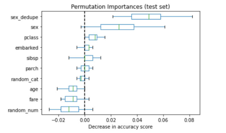
For instance this, let’s use an excessive instance and duplicate the column intercourse to retrain the mannequin.
RF practice accuracy: 0.794
RF check accuracy: 0.802
The mannequin efficiency barely decreases as we added a characteristic that didn’t add any data.
We see now the significance of the intercourse options are actually distributed between two duplicated intercourse columns. What occurs if we add a little bit of noise to the duplicated column?
Let’s strive including random noise starting from 0–1 to the intercourse.

sex_noisy is now an important variable. What occurs if we improve the magnitude of noise added? Let’s improve the vary of the random variable to 0–3.

Now we are able to see with extra noise added, that sex_noisy now not ranks as the highest predictor and intercourse is again to the highest. The conclusion is that permutation importances computed on a random forest mannequin unfold significance throughout collinear variables. The quantity of sharing seems to be a operate of how a lot noise there may be between the 2.
Coping with Collinear Options
Let’s check out the correlation between options. We use feature_corr_matrix from the rfpimp package deal, which supplies us Spearman’s correlation. The distinction between Spearman’s correlation and commonplace Pearson’s correlation is that Spearman’s correlation first converts two variables to rank values after which runs Pearson correlation on ranked variables. It doesn’t assume a linear relationship between variables.
feature_corr_matrix(X_train)

from rfpimp import plot_corr_heatmap
viz = plot_corr_heatmap(X_train, figsize=(7,5))
viz.view()

pclass is extremely correlated with fare, which isn’t too stunning as class of cabin relies on how a lot cash you pay for it. It occurs very often in enterprise that we use a number of options which are correlated with one another within the prediction mannequin. From the earlier instance, we see that when two or a number of variables are collinear, the importances computed are shared throughout collinear variables based mostly on the information-to-noise ratio.
Technique 1: Mix Collinear Function
One solution to deal with that is to mix options which are extremely collinear with one another to type a characteristic household and we are able to say this characteristic household collectively ranks because the X most necessary. To try this, we are going to use the rfpimp package deal that permits us to shuffle two variables at one time.

Technique 2: Take away Extremely Collinear Variable
If a characteristic relies on different options, which means the options could be precisely predicted utilizing all different options as impartial variables. The upper the mannequin’s R² is, the extra dependent characteristic is, and the extra assured we’re that eradicating the variable received’t sacrifice the accuracy.

The primary column dependence reveals the dependence rating. A characteristic that’s utterly predictable utilizing different options would have a price near 1. On this case, we are able to in all probability drop one of many pclass and fare with out affecting a lot accuracy.
As soon as we 1)have a sturdy mannequin and implement the proper technique to calculate permutation significance and a couple of)take care of characteristic correlation, we are able to begin crafting our message to share with stakeholders.
For the widespread query individuals ask “Is characteristic 1 10x extra significance than characteristic 2?”, it’s possible you’ll perceive at this second that now we have the arrogance to make the argument solely when all of the options are impartial or have very low correlation. However in the actual world, that’s hardly ever the case. The really useful technique is to assign options to the Excessive, Medium, and Low affect tiers, with out focusing an excessive amount of on the precise magnitude. If we have to present the relative comparability between options, attempt to group collinear options (or drop them) to characteristic acquainted and interpret based mostly on the group to make the argument extra correct.
You will discover the code on this article on my Github..
[1] Beware Default Random Forest Importances
[2]Permutation Significance vs. Random Forest Significance (MDI)
[3]Function Importances for Scikit-Study Machine Studying Fashions
[4]The Arithmetic of Choice Tree, Random Forest Function Significance in Scikit-learn and Spark
[5]Explaining Function Significance by instance of a Random Forest
