The way to make an equal elastic web regression between sklearn and Tensorflow in Python
This text is meant for the practitioners who wish to examine the sklearn and Keras implementation of elastic web regression. Primarily, go from Sklearn loss perform to Keras (Tensorflow) loss perform.
Most important components of the article:
- A quick introduction to regularization in regression.
- Sklearn implementation of the elastic web.
- Tensorflow implementation of the elastic web.
- Going from one framework to a different.
- Writing a customized loss perform.
- Evaluating the outcomes.
All of the codes are in my repository: https://github.com/Eligijus112/regularization-python
Regression is a course of in machine studying figuring out the connection between the imply worth of the response variable Y and options X.
The prediction for a mannequin is denoted as y with a hat and is calculated by estimating the coefficients beta from knowledge:
The betas with no hat denote the theoretical mannequin and the betas with a hat denote the sensible mannequin, which was obtained utilizing the observable knowledge. How will we calculate the coefficients beta?
The calculation begins with defining an error. An error reveals how a lot a prediction differs from the true worth.
We’d clearly just like the error to be as small as doable as a result of that will point out that our discovered coefficients approximate the underlying dependant variable Y the very best given our options. Moreover, we wish to give the identical weight to each the adverse and constructive (amongst different causes) errors thus we’ll introduce the squared error time period:
In a regular linear regression, our aim is to attenuate the sq. error alongside all of the observations to a minimal. Thus, we are able to outline a perform known as imply squared error:
The x and y knowledge are mounted — we can’t change what we observe. The one leverage we now have is to attempt to match completely different beta coefficients to our knowledge to get the MSE worth as little as doable. That is the general aim of linear regression — to attenuate the outlined loss perform to a minimal utilizing solely the beta coefficients.
With a view to reduce the MSE worth, we are able to use varied optimization algorithms. Some of the well-liked algorithms is stochastic gradient descent or SGD for brief.
The gradient half is that we calculate the partial derivatives by way of all coefficients:
The descent half is that we iteratively replace every coefficient beta:
The M is the variety of iterations.
The alpha fixed is a constructive worth, known as the educational fee.
The stochastic half is that we don’t use all of the samples within the dataset in a single iteration. We use a subset of knowledge, additionally known as a mini-batch, when updating the coefficients beta.
Regularization in regression is a technique that avoids constructing extra advanced fashions, in order to keep away from the danger of overfitting. There are numerous forms of regularization, however three of the preferred ones are:
We regularize by including sure phrases to the loss perform which we optimize. Within the case of Lasso regression, the normal MSE turns into:
We add the sum of absolute coefficient values within the new loss perform. The larger absolutely the sum of the coefficients, the upper the loss. Thus, when optimizing, the algorithm will get penalized for giant coefficients.
Ridge regression places a good greater coefficient penalty as a result of the magnitude will get squared. One disadvantage of ridge regression is that such a regression doesn’t set any coefficients to 0, whereas lasso can be utilized for characteristic discount, as a result of it could actually set among the coefficients to zero.
Elastic web combines each ridge and lasso regression. Lambda values normally vary between 1 and 0.
Now that we now have a short theoretical overview out of the best way, we are able to transfer on to the sensible components. The information we’ll use is taken from Kaggle¹ concerning home gross sales within the US from 2014 to 2015.
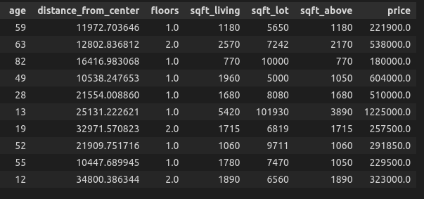
We’ll attempt to clarify the worth of a home utilizing the 6 options obtainable.
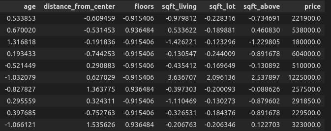
We’ll standardise the options. On this article, I wish to showcase the comparability between TensorFlow and Sklearn, thus I will not spend a lot time characteristic engineering the dataset.
Allow us to strive the Sklearn implementation of Elastic Internet
https://scikit-learn.org/secure/modules/generated/sklearn.linear_model.ElasticNet.html
The loss perform utilized in Sklearn is:
Allow us to set alpha = 1 and lambda (known as l1 ratio in Sklearn) to 0.02.
# Becoming the mannequin to knowledge utilizing sklearn
el = ElasticNet(alpha=1.0, l1_ratio=0.02)
el.match(d[features], d[y_var])# Extracting the coefs
coefs = el.coef_# Making a dataframe with the coefs
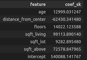
coefs_df = pd.DataFrame({‘characteristic’: options, ‘coef_sk’: coefs})# Appending the intercept
coefs_df = coefs_df.append({‘characteristic’: ‘intercept’, ‘coef_sk’: el.intercept_[0]}, ignore_index=True)
The ensuing coefficient knowledge body is:
Tensorflow is a very fashionable deep studying community. The framework lets us use the elastic web regularization as effectively utilizing the L1L2 class https://keras.io/api/layers/regularizers/#l1l2-class.
Allow us to examine two formulation — the sklearn one and TensorFlow.
Scikit study:
Tensorflow:
As we are able to see, TensorFlow doesn’t divide the MSE a part of the equation by 2. With a view to have comparable outcomes, we have to create our personal customized MSE perform for TensorFlow:
After writing this tradition loss perform, we now have the next equation:
Now we are able to equalize each equations and attempt to create formulation for lambda 1 and lambda 2 in TensorFlow by way of alpha and lambda from sklearn.
Thus we’re left with:
A perform to rework sklearn regularization to TensorFlow regularization parameters:
Now let’s put every part collectively and practice a TensorFlow mannequin with regularization:
# Defining the unique constants
alpha = 1.0
l1_ratio = 0.02# Infering the l1 and l2 params
l1, l2 = elastic_net_to_keras(alpha, l1_ratio)# Defining a easy regression neural web
numeric_input = Enter(form=(len(options), ))
output = Dense(1, activation=’linear’, kernel_regularizer=L1L2(l1, l2))(numeric_input)mannequin = Mannequin(inputs=numeric_input, outputs=output)
optimizer = tf.keras.optimizers.SGD(learning_rate=0.0001)# Compiling the mannequin
mannequin.compile(optimizer=optimizer, loss=NMSE(), metrics=[‘mse’])# Becoming the mannequin to knowledge utilizing keras
historical past = mannequin.match(
d[features].values,
d[y_var].values,
epochs=100,
batch_size=64
)
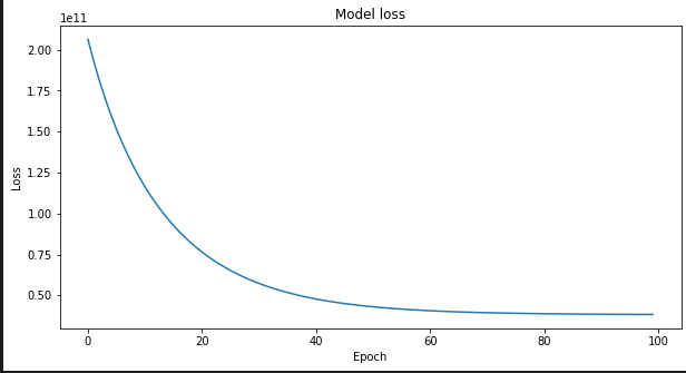
When the alpha = 1.0 and l1 ratio is 0.02, the constants for TensorFlow regularization are 0.02 and 0.49.
The coaching appears to be like easy:
The TensorFlow and sklearn regression coefficients:
# Creating the coef body for TF
coefs_df_tf = pd.DataFrame({
‘characteristic’: options + [‘intercept’],
‘coef_tf’: np.append(mannequin.get_weights()[0], mannequin.get_weights()[1])
})## Merging the 2 dataframes
coefs_df_merged = coefs_df.merge(coefs_df_tf, on='characteristic')coefs_df_merged['percent_diff'] = (coefs_df_merged['coef_sk'] - coefs_df_merged['coef_tf']) / coefs_df_merged['coef_sk'] * 100
The ensuing knowledge body is:
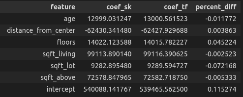
The coefficients differ by a really small quantity. This is because of the truth that below the hood, sklearn and TensorFlow provoke the coefficients with completely different features, some randomness is concerned and we are able to all the time tune the epochs and batch measurement to get nearer and nearer outcomes.
On this article we:
- Had a short introduction to regularization.
- Created a customized TensorFlow loss perform.
- Created a perform that mimics sklearn regularization in TensorFlow.
- Created and in contrast two fashions.
Blissful studying and coding!
