
Some suspicious factors are sometimes wrongly decreased to outliers. Different varieties together with their detection instruments deserve consideration.

Context
“Rubbish in, rubbish out”
This sentence outlines the consequence of middling knowledge on the mannequin’s end result. Throughout a undertaking, an indispensable step is to carry out EDA (Explanatory Knowledge Evaluation) to test, inter alia, the “cleanliness” of their knowledge. With out this step, somebody might invalidate outcomes and ask for sturdy evaluation, that’s, evaluation that offers with uncommon observations.
A standard strategy recurrently executed is to analyze the univariate distribution of every variate through boxplots and scatterplots. In addition to giving noticeable conclusions, these methods could be meaningless in a multivariate context and might’t inform us how this subset of surprising knowledge impacts the estimated mannequin.
Moreover, masking all uncommon factors within the time period “outliers” is inappropriate. Certainly, totally different sorts of factors may affect the estimated mannequin in their very own means.
For that reason, along with “outliers”, 2 different terminologies will likely be launched: excessive leverage, and influent. Subsequent half, every terminology will likely be clarified together with examples.
Terminology
In a regression evaluation, these phrases are associated in addition to they’ve totally different meanings:
- Influential level: a subset of the info having an affect on the estimated mannequin. Eradicating it seems to modify considerably the outcomes of the estimated coefficient.
- Outlier: an remark that falls outdoors the overall sample of the remainder of the info. In a regression evaluation, these factors stay out of the arrogance bands on account of excessive residual.
- Excessive Leverage: an remark that has the potential to affect predominantly the expected response. It may be assessed by ∂y_hat/∂y: how a lot the expected response differs if we shift barely the noticed response. Usually, they’re excessive x-values.
Earlier than going deeper, let’s give trivial examples to get the gist.
Examples

Comment: Justifications will likely be executed graphically even when constant analyses require statistical conclusion (R², p-value, normal deviation)
a.
Influent: Each regression traces aren’t tremendously totally different with an identical estimated slope and a comparatively shut estimated intercept=> NO
Outlier: Does the pink level appears to have a excessive residual? Sure, and it’s undoubtedly out of the linear sample => YES
Excessive Leverage: Is it an excessive x worth? If we transfer barely the pink level alongside the y-axis, does the expected response will shift significantly? The purpose is near the imply x-values and a y-variation is not going to extremely modify the expected response => NO
b.
Influent: Each regression traces are virtually overlapping => NO
Outlier: The pink level obeys the linear sample and has a low residual => NO
Excessive Leverage: With this excessive x-value, the pink level could be within the lengthy tail of the distribution. Moreover, as proven within the following graph, when the purpose is barely moved upward, the expected response varies altogether => YES
c.
Influent: Because the pink level determines absolutely the regression line, it’s clearly influential => YES
Outlier: The remainder of the info doesn’t observe a common sample, subsequently, with this configuration, we are able to’t infer a possible outlier =>?
Excessive Leverage: As being the primary influential level, a variation on the noticed response impacts extraordinarily the expected response => YES
As this level is influential, you need to be deeply suspicious of the estimate.
d.
This one is a mix of examples a) and b). It’s a excessive leverage outlier. Moreover, each regression traces are extra distant opposite to the 2 first instances. It’s an influential level.
What can we study from these examples?
In actuality, influential factors are essential as they appear to have a disproportionate affect on the estimated mannequin. An influential level seems to be each an outlier and a excessive leverage level. That’s, an out-of-distribution pattern each within the subspace of the x-values (excessive leverage) and y-values (outliers) will significantly affect the estimated mannequin.
Eradicating these suspicious factors and analyzing the statistical outcomes prove to identify these influential factors.
Nevertheless, every little thing has been described in an ideal world the place there may be merely one variable however actual issues embody a number of variables. For instance, excessive leverage factors aren’t merely excessive x-values however could be a singular mixture of x-values that make these factors removed from different observations within the subspace of the explanatory variables.
The following half is the generalization of the final half with a number of predictor values. I’ll present statistical instruments to effectively detect such factors and characterize them.
The “Hat” Matrix
In a number of linear regression, the idea states that the expected response could be immediately associated to the noticed response:

The matrix H, additionally referred to as the “hat matrix”( as a result of it provides the “^” to the y), is the central notion to detect suspicious factors. Just by multiplying y by this matrix, we have now immediately the expected response, and H is just a operate of X.
For a greater understanding, the final equality could be written as the next equations:

At this stage, we have now outlined an indispensable factor: h_ii. As we’ll see later, this factor exists in each method associated to uncommon level detection. Extra exactly, it has a reputation: the leverage! Certainly, in the event you recall the earlier definition, the leverage could be estimated by ∂y_hat/∂y, which is precisely h_ii.

Now, I can even introduce the idea of residual. As you think about, residuals — the distinction between the expected and the noticed response — are decisive within the detection of outliers. We are able to show the next outcomes:

Three helpful penalties derive from this end result:

Comment: Every residual has a definite variance and they’re mutually correlated.
Since we have now laid the foundations for the idea, let’s current the instruments to characterize questionable factors.
Excessive Leverage
As I’ve already talked about, the leverage is the worth h_ii which defines the coefficient that multiplies the i-th noticed response when calculating the i-th predicted response. Thus, it stands to motive that excessive leverage = excessive h_ii, proper? However what threshold is related to think about the h_ii as excessive?
The chosen cutoff is predicated on a rule of thumb: if h_ii is bigger than 2 instances the imply of the h_ii, the i-th remark is considered as excessive leverage. The imply could be rewritten as proven under:

It’s value mentioning that this situation is a rule of thumb, nothing rigorous. You may encounter one other threshold elsewhere (typically 3 instances the imply if n is comparatively giant)
Studentized Residuals For Outliers
Outliers are, by definition, excessive residuals factors. Nevertheless, every residual has a definite variance. Thus, to make rigorous analyses, a standardization of the residuals have to be achieved. In that means, residuals could be quantified in normal unit deviations after which, in contrast. Therefore the next relation:

Nevertheless, a recurring challenge in regression evaluation is the existence of the σ. This amount is launched within the definition of the mannequin as the usual deviation of the error time period. Nevertheless, as its worth is never out there, an estimator is required.

s² is an unbiased estimator of σ². Nevertheless, with mathematical instruments, we are able to show that t_i does not observe a t-student distribution. To acquire this distribution, we have now to merely take away the i-th remark within the estimator such that:

s_i denote the MSE of the mannequin with out the i-th remark. If we intend to compute s_i for each i, we should refit the mannequin each time. Fortuitously, the equality above resolves that challenge as a result of s_i is a operate of variables that don’t must take away the i-th remark.
After getting all these studentized residuals, how will we assess outliers?
Plots are typically one of the best ways to grasp and signify visually outliers:
- Studentized Residuals vs Predicted Observations with a threshold of two or 3 (in absolute worth) to label outliers (Furthermore, we should always see a uniform distribution as a result of, theoretically, the covariance between each the residual and the expected response vector is null)
- Studentized Residuals vs Commentary Id with additionally a threshold of two or 3. This plot is beneficial with time-series knowledge. Certainly, it may possibly result in outliers detection associated to the time element.
Prepare dinner Distance and DFFITS For Influential Factors
By definition, influential factors have an effect on considerably the estimated mannequin and the related outcomes. A simple concept might be to take away every level, refit the mannequin, and analyze discrepancies between the “full” mannequin and the mannequin with out the eliminated level. As at all times, we have to outline a measure to tell how a lot the purpose is influential.
On this article, I’ll current two indicators: the Prepare dinner Distance and DFFITS.
By definition, Prepare dinner Distance is outlined by the primary equality. The 2nd equality stems from the first equality and is usually extra sensible:

The (2) equality exhibits immediately the hyperlink between influential factors, excessive leverage factors, and outliers.
Certainly, D_i is operate of: t_i and h_ii/(1-h_ii). Each phrases quantify respectively outliers and excessive leverage factors. Furthermore, h_ii/(1-h_ii) is an rising operate of h_ii. Consequently, the upper |t_i| and/or h_ii are, the upper the prepare dinner distance is. It confirms what we beforehand stated: if an remark is a excessive leverage outlier, it’s actually an influential level too.
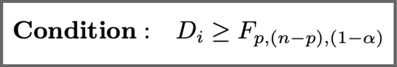
A statistical threshold to find out if the purpose is influential:
DFFITS and Prepare dinner Distance are virtually the identical:

