
Making an animation to seek out the very best stability between x and y coordinates on a curve
I used to be lately requested to assist with a mission that concerned discovering the x and y values on a curve that had the biggest space beneath them. To perform this, determined to make this animation:
Other than trying fairly cool, such a job can have utility in analysis or business. As one variable will increase, the opposite decreases, and so that you need to discover the values of x and y that present the utmost space below the curve that maps their relationship (I name this the very best x/y trade-off).
The instance within the preliminary downside I helped with was within the context of rising fruits in a greenhouse with warmth capability on the x-axis and frequency/yr on the y-axis. One other instance might be between warmth and strain in a bioreactor or meals processing system— maximising one or each of them could be too expensive, so discovering the very best trade-off between the 2 could be fascinating.
For the reason that downside was enjoyable and never too troublesome, I assumed I’d make an article out of it for others to be taught from. After I began Python, one thing that pissed off me typically was the assumed data of a lot of the code I discovered on-line. To keep away from this, I’m going to attempt to be as complete as doable when explaining my code and present a number of methods of attaining the identical objective.
I like to recommend studying the contents under and skipping over bits you’re extra aware of to get to the bits you’ll profit from. I’ll import libraries as we use them so that you get a greater sense of how and after they’re used. With that, let’s start!
Contents:
- Making a dataframe
- Eradicating outliers
- Coping with not out there (NA) values
- Make a spline curve
- Discover greatest x/y trade-off
- Plotting
- Animating
Making a dataframe
The information used within the unique mission is personal, so as an alternative, I made some information of a really related nature for this text. It additionally means you possibly can copy and paste it simply and comply with alongside.
Now, let’s put the information right into a dataframe since it is going to make future steps a bit of simpler for us and since dataframes are one of the vital widespread information sorts you’ll come throughout in Python.
We are able to do that by specifying a dictionary (utilizing the curly brackets {}) with the specified column names earlier than the colon and the information we’re utilizing after:
This throws an error that tells us that we will’t do that due to the scale of the information.
They’re each arrays, however x is a 1D array whereas y is a 2D array by which every of the 17 components can also be an array. We are able to see this utilizing .form :
and likewise by printing a given worth of x in comparison with y:
This makes y a bit of bit extra awkward to cope with. To repair this, let’s shortly loop by y and add all of the values to an empty checklist, new_y, so now we have the information in a extra usable kind.
Right here, so loop by every worth of y and from every array take the primary (and solely) worth by utilizing [0]. Then we append this to the brand new empty checklist we simply made.
Now, we will make a dataframe from the information:
Eradicating outliers
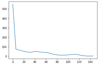
The presence of outliers in information is all too widespread and may at all times be investigated. This may be completed with visible inspection if the information is small, as in our case.
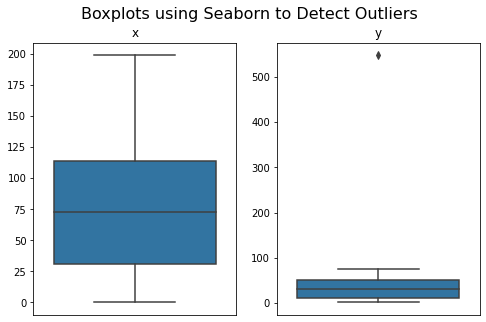
Another choice us utilizing approaches like boxplots. I just like the seaborn bundle for this objective:
One other approach to examine for outliers is to make use of an outlier operate. Beforehand, those I discovered on-line didn’t fulfill my wants, so I made a decision to make my very own.
It takes a dataframe as the primary argument and a z worth because the second argument, loops by the columns, and columns with outliers, their values, and their location within the dataframe to you.
For conciseness, I pass over the code for outlining the outlier operate, however you possibly can copy it from this hyperlink.
As we noticed with the boxplots, we see that y has an outlier at index place 0 of worth 548.
What I like about this outlier operate in comparison with others is it doesn’t simply take away them however presents them to you and allows you to resolve what to do with them. That is handy in my work as a result of usually I’ve outliers in my information that shouldn’t be eliminated, reminiscent of excessive body-mass index values that, though outliers, mirror real readings and shouldn’t be excluded with out good cause.
On this case, although, it’s doable that the primary worth represents one thing like vitality required to begin up the system and this vitality couldn’t be sustained all through the entire course of, due to this fact representing a real outlier. That is supported by the truth that it happens throughout the first millisecond of recording.
Having the information in dataframe kind now makes eradicating this datapoint simpler since, as an alternative of getting to take away each x and y values, we will simply take away the entire row. This makes issues handy on bigger datasets and prevents the chance of eradicating datapoints in several positions, inflicting an information shift.
There are numerous methods to do that.
We are able to copy the index worth from the outlier report and drop that index worth like this:
One other state of affairs could be to take away any row with a sure studying.
I encountered this lately with steady blood glucose monitoring information the place common calibrations offered unrealistic readings of a hard and fast quantity. If this, in our case, was 548, we may use this code to eliminate all situations the place the y worth is the same as 548:
And it might even be that 548 represents a minimize off of some type, the values above which aren’t sensible and due to this fact might be discarded as outliers. The next code can do that:
A remaining possibility on this case although, since our outlier is the primary worth within the dataframe, is simply to utilizing indexing to take away the primary worth:
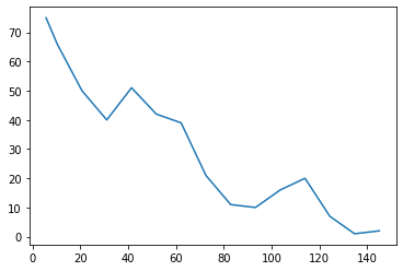
Now, the information appears to be like extra affordable:
Coping with not out there (NA) values
One other vital a part of information cleansing is checking for NA values. We is perhaps deceived that our information doesn’t include NA values since we have been capable of plot it utilizing matplotlib above.
Sure capabilities simply ignore NA values and nonetheless work (like matplotlib and seaborn above), however others just like the operate we are going to use under is not going to work with NA values.
We must always at all times examine. Since our information is in a dataframe kind, pandas’ isna() is the easiest way to do this. The operate isna() returns every merchandise of the dataframe as a Boolean (True or False) as as to if it’s or shouldn’t be an NA worth.
This isn’t notably useful generally, however by combining this with sum() to see the NA values per column and sum().sum() to see the variety of NA values in whole within the dataframe, it turns into much more helpful.
Earlier than simply coping with NA values, we’d need to examine them a bit of first. The primary, second, and third strains of code
respectively.
This NA worth might be one thing like a price so low that it’s now not detected, one thing I come throughout fairly often in information I’m working with. It might be applicable to swap this to 0, nevertheless as a result of we’re unsure, we are going to drop the information as an alternative.
Make a spline curve
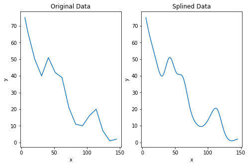
After we plot our information we see that it’s jagged and never clean. There are numerous methods for curve smoothing however I’ve good expertise with scipy’s make_interp_spline.
The x and y information are given as inputs to estimate coefficients for a curve. We then cut up the x information up into many particular person and evenly spaced factors utilizing numpy’s linspace operate and use this to estimate the values for y.
Now, if we plot this information, we see it’s clean while nonetheless representing the approximate form of the information.
It’s price noting that points can come up after we modify the information on this means. For instance, let’s say we positioned our NA worth with a 0 as we thought of, the information would appear like this as an alternative:

In our case, this difficulty arises as a result of the y worth at x=145 is barely greater than the information level earlier than it, though since each the values are small this might merely resulting from measurement variations moderately than something meaninful. Other than this, the information is nicely represented, although this serves as a reminder to at all times examine that splined information represents the noticed information.
Discover greatest x/y trade-off
On this case, the splined information shouldn’t be solely useful for us for plotting nevertheless it additionally helps us with our subsequent step: discovering the values of x and y that can give us the biggest space below the curve (AUC). Now, as an alternative of getting 14 information factors as within the unique dataset, now we have 500 (or nevertheless many we determined to specify within the third argument of the np.linspace operate.
By rephrasing this query as discovering out an space, and by realizing that the underside left nook of the rectangle is mounted at 0,0, the highest left is mounted at 0,y, the underside proper is mounted at x,0, and the highest proper is each level on the road, the query turns into a easy multiplication.
First, we will calculate the world for all of the factors that compose the curve by making a dataframe with the splined information after which including a brand new column to symbolize space:
Then we discover the max row within the dataframe:
We are able to then save these coordinates to 2 new variables with the next code:
and now we’re able to visually symbolize this on our new smoothed curve.
Plotting
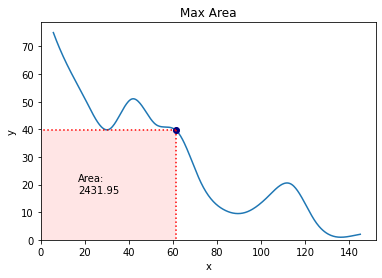
There is perhaps varied methods so as to add a rectangle to a graph as we need to do in matplotlib however the way in which I discovered most easy was with a bundle referred to as mpatches.
We create 2 new variables which symbolize the coordinates of the underside left nook of the rectangle, after which 2 which symbolize the peak and width. Since our rectangle will begin at 0,0 (the origin), then the primary 2 variables are 0 and 0. The peak and width are then merely the values we obtained for x and y, i.e., bestx and besty.
We then use the mpatches bundle to create a rectangle of the proportions we simply specified and the design we want.
I included varied arguments that can be utilized right here to change the looks of the rectangle and put some explanations for what they do afterwards, however there are additionally different arguments that permit manipulation of the rectangle look which you could discover.

It appears to be like fairly cool (that is what classifies as cool for nerds), however we will simply make it a bit of bit cooler.
We are able to add the purpose on the graph which corresponds to greatest x and greatest y to emphasize this a bit of extra. We may additionally think about including some strains taking place from the purpose to the x and the y to emphasize every of those values a bit of extra, too. We are able to obtain this simply with the next code:

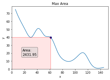
We may additionally add some textual content if we so wished. A logical entry right here could be the world of the rectangle:
To make the textual content stand out a bit extra, we are going to add a field round it. We may even make the font a bit of larger.
Animating
Including the ending touches to all of that is now to animate our plot in a means that exhibits the world of every level on the curve ranging from the primary level to the final.
There are a number of methods and packages to animate plots in Python however I discovered this from Christopher Tao essentially the most easy approach to do it.
It entails making separate plots for every level on the curve after which merging them right into a GIF utilizing a bundle referred to as Imageio. It’s most likely not essentially the most environment friendly means to do that nevertheless it’s fairly easy and never technical.
I’ll construct the code bit-by-bit and clarify every chunk as we go, then put all of it collectively so you possibly can copy and paste it and use it simply. (I don’t advocate working every code little by little since you’ll find yourself with numerous photographs in your listing).
The very first thing we are going to do is loop by the splined_df and make a brand new plot for ever single information level. The primary adjustments we have to make to do that is 1) change the width and top for the field from bestx and besty to the x and y values of the present information level, and a couple of) do the identical for the purpose and the vlines and hlines. That is simple:
Subsequent, we’re going to replace the textual content field to point out the world of the present datapoint. It doesn’t make sense to maintain the textual content field exhibiting the world of the field in the identical place as within the earlier figures because the field shall be altering in form and dimension. As a substitute, let’s put it out of the way in which within the high proper nook:
Moreover, what could be cool is to point out how the utmost space adjustments alongside the curve. For this, we are going to create one other textbox simply beneath that exhibits the present greatest space up till now.
To do that, we have to create a variable outdoors of the for loop firstly of this part and set it to a quantity decrease than our lowest worth. In our case, this might be 0, nevertheless it’s good apply to set this quantity to be unfavourable infinity simply in case we’re ever working with information with very low or very low (and unknown) information factors.
Subsequent, we then make an if/else clause inside our for loop to say: if the world of the present information level is largest than the earlier one, then the present information level now turns into current_max and we print this within the textbox. Else — if the present information level shouldn’t be bigger than the worth for current_max — then we simply print current_max within the textbox (i.e., it’s unchanged from the final image). We’ll additionally spherical the world to 1 decimal place to keep up readability.
This appears to be like like this:
Lastly, we save every particular person determine and shut the plot to cease it every one from popping up in whichever setting you’re working Python.
All of the figures will exist in your listing with the identify “max_area” adopted by the variety of the row within the splined_df dataframe.
The ultimate step is to make use of the library imageio to make all our photographs right into a GIF. The next code does this by looping by all the photographs we simply saved and writing them into one GIF.
After a few minutes, you’ll have your animation.
The ultimate step is to delete all of the recordsdata we simply made, leaving solely the GIF. This may be completed with the next code:
Under, the complete code for making the anaimation with the intention to copy and paste it to make use of in your personal information.
I hope you discovered this useful and are capable of apply or adapt the code to supply one thing related to what you could do!
