
As a result of unhealthy information results in unhealthy fashions

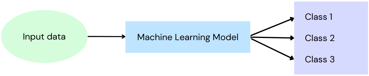
Basically, a machine studying mannequin is one thing that configures itself to foretell an final result, primarily based on the coaching information. When you feed the mannequin coaching information that doesn’t characterize the info the mannequin will face when truly getting used, you can’t anticipate something however flawed predictions. This text gives you insights on creating a superb dataset that is ready to characterize information the mannequin will face when it’s being utilized in the true world.
However earlier than we begin constructing nice datasets, first, we should perceive the parts of a dataset (lessons, labels, options, and have vectors). Then, we are going to transfer on to information preparation. That is the place we deal with lacking options and scale options. Subsequent, we talk about why and the way we should always partition the dataset. Lastly, we are going to take a look at why we should always have a closing look at our information and find out how to discover issues that would nonetheless exist, equivalent to outliers and mislabeled information.
Let’s get began.
Courses and Labels
In classification duties, the enter options are mapped to discrete output variables. For instance, by contemplating the enter information, the mannequin predicts whether or not the output is a “canine”, “cat”, “horse” and many others. These output variables are outlined as lessons. An identifier referred to as a label is given to every enter within the coaching information to characterize these lessons.
To a mannequin, the inputs are simply numbers. A mannequin doesn’t care or know the excellence between a picture of a canine or a voice pattern. This additionally applies to the labels. Because of this, lessons could be represented in any means we wish. In observe, we frequently use integer values beginning with 0 to map the labels to their respective class. An instance is proven beneath.
┌───────┬────────────┐
│ Label │   Class    │
├───────┼────────────┤
│     0 │ particular person     │
│     1 │ bicycle    │
│     2 │ automotive        │
│     3 │ bike │
│     4 │ airplane   │
│     5 │ bus        │
│     6 │ prepare      │
│     7 │ truck      │
│     8 │ boat       │
│     9 │ site visitors    │
└───────┴────────────┘
The desk is an exerpt from the COCO dataset, displaying its lessons and labels.
Within the above instance, each enter that represents a bicycle is labeled 1 and each enter representing a ship is labeled 8. It’s possible you’ll now surprise, what precisely are we labeling? What is definitely the enter of an individual or a ship? That is the place the all-important options are available in.
Options and Function Vectors
Options are the inputs utilized by the mannequin to provide a label as output. These are numbers, as talked about above, and characterize various things relying on the duty. For instance, within the iris dataset which incorporates information about three species of Iris flowers, the options are the size of the sepals and petals.
The 4 obtainable options within the iris dataset for the iris flower species often known as Setosa are proven beneath.
(solely the primary 5 rows of the dataset are proven)    Sepal.Size  Sepal.Width  Petal.Size  Petal.Width   Species
1          5.1          3.5           1.4          0.2    setosa
2          4.9          3.0           1.4          0.2    setosa
3          4.7          3.2           1.3          0.2    setosa
4          4.6          3.1           1.5          0.2    setosa
5          5.0          3.6           1.4          0.2    setosa
Notice: The lessons within the above dataset are the completely different species of Iris flowers, Setosa, Virginica, and Versicolor with labels 0, 1 and a couple of given to those lessons respectively.
Thus, options are merely the numbers that we are going to use as inputs to the machine studying mannequin. When the machine studying mannequin is skilled, the mannequin learns relationships between the enter options and the output labels. We make an assumption right here that there truly is a relationship between the options and the labels. In instances the place there aren’t any relationships to study, the mannequin could fail to coach.
As soon as coaching is concluded, the realized relationships are used to foretell output labels of enter characteristic vectors (units of options given as enter) with unknown class labels. If the mannequin continues to make unhealthy predictions, a cause is likely to be that the options used to coach the mannequin weren’t enough sufficient to establish a superb relationship. That is why selecting the right options issues at first of any machine studying undertaking. Extra data on selecting good options and why unhealthy options ought to be ignored could be present in my publish beneath.
Options could be of various sorts, equivalent to floating level numbers, integers, ordinal values (pure, ordered classes the place the distinction between values usually are not all the time the identical), and categorical values (the place numbers are used as codes, e.g male=0 and feminine=1).
Recap: options are numbers that characterize one thing we all know, that may assist construct a relationship to the output label. Check out some rows of the Iris dataset beneath, now displaying all parts, options class and labels. Every row containing all 4 options is one characteristic vector.
                      Options
________________|_____________________       Class   Label
|                                      |        |       |
Sepal.Size  Sepal.Width  Petal.Size  Petal.Width  Species
5.1          3.5           1.4          0.2       setosa     0
7.1          3.0           5.9          2.1       virginica  1
4.7          3.2           1.3          0.2       setosa     0
6.5          3.0           5.8          2.2       virginica  1
6.9          3.1           4.9          1.5       versicolor 2
Now that we’ve got a superb grip on what a dataset incorporates, there are two necessary issues to think about earlier than we begin constructing our nice dataset:
- Learn how to deal with lacking characteristic values
- Function Scaling
Coping with lacking options
It’s possible you’ll come throughout instances the place there are lacking options in your information, for instance, you will have forgotten to make a measurement, or some information for a pattern has been corrupted. Most machine studying fashions do not need the flexibility to simply accept lacking information, so we should fill in these values with some information.
There are two approaches you possibly can absorb such situations. You could possibly both add a price that falls far outdoors the characteristic’s vary with the premise that the mannequin can pay much less significance to it or, use the imply worth of the options over the info set rather than the lacking worth.
Within the instance beneath, some options are lacking, indicated by clean areas.
Sepal.Size  Sepal.Width  Petal.Size  Petal.Width  Label
5.1          3.5           1.4                      0
7.1                        5.9          2.1         1
4.7          3.2                        0.2         0
3.0           5.8          2.2         1
6.9          3.1           4.9          1.5         2
The imply for all of the options is calculated and proven within the desk beneath
Sepal.Size  Sepal.Width  Petal.Size  Petal.Width
5.95         3.2           4.5          1.5
By changing the lacking values with the imply values, we are able to receive a dataset that can be utilized to coach a mannequin. This isn’t higher than having actual information however ought to be ok to make use of when information is lacking. An alternate if the dataset is massive sufficient is to make use of the mode (most occurring worth) by figuring out it by means of a generated histogram.
Function scaling
Oftentimes, characteristic vectors which are made of various options can have a number of completely different ranges. For instance, whereas a set of options will probably be between 0 and 1, one other characteristic can have values between 0 to 100,000. One other will probably be between -100 to 100. Because of this, some options will dominate others due to their bigger vary, which causes the mannequin to endure in accuracy. To beat this drawback, characteristic scaling is used.
To know this idea in addition to to strengthen what we realized within the above sections, we are going to create an artificial information set and take a look at it.
┌────────┬─────┬──────┬──────┬───────────┬────────┬───────┐
│ Pattern │ f1  │  f2  │  f3  │    f4     │   f5   │ Label │
├────────┼─────┼──────┼──────┼───────────┼────────┼───────┤
│      0 │  30 │ 3494 │ 6042 │  0.000892 │ 0.4422 │     0 │
│      1 │  17 │ 6220 │ 7081 │ 0.0003064 │ 0.5731 │     1 │
│      2 │  16 │ 3490 │ 1605 │ 0.0002371 │   0.23 │     0 │
│      3 │   5 │ 9498 │ 7650 │ 0.0008715 │ 0.8401 │     1 │
│      4 │  48 │ 8521 │ 6680 │ 0.0003957 │ 0.3221 │     1 │
│      5 │  64 │ 2887 │ 6073 │ 0.0005087 │ 0.6635 │     1 │
│      6 │  94 │ 6953 │ 7970 │ 0.0005284 │ 0.9112 │     0 │
│      7 │  39 │ 6837 │ 9967 │ 0.0004239 │ 0.4788 │     1 │
│      8 │  85 │ 9377 │ 4953 │ 0.0003521 │ 0.5061 │     0 │
│      9 │  46 │ 4597 │ 2337 │ 0.0004158 │ 0.8139 │     0 │
└────────┴─────┴──────┴──────┴───────────┴────────┴───────┘
The primary column is the pattern quantity.
Every row of a pattern is an enter to the mannequin, given as a characteristic vector.
A characteristic vector is represented by 5 options for every pattern
- characteristic set is {f1, f2, f3, f4, f5}
- Sometimes the total characteristic vector is refered to with the uppercase letter (F).
- Function vector for pattern 3 could be refered to as F3.
One characteristic vector is highlighted in daring for pattern 2 within the desk.
The final column is the label. There are two lessons, represented by the labels 0 and 1.Discover how samples begin with 0. It is because we work with Python and Python is 0 listed.
Now to the scaling half. You may see in our artificial information desk that completely different options have completely different ranges. Let’s take a look at all of the options and think about their minimal, most, common, and vary values.
┌──────────┬───────────┬───────────┬──────────┬────────────┐
│ Function  │   Vary   │  Minimal  │ Most  │  Common   │
├──────────┼───────────┼───────────┼──────────┼────────────┤
│ f1       │        89 │         5 │       94 │       44.4 │
│ f2       │      6611 │      2887 │     9498 │     6187.4 │
│ f3       │      8362 │      1605 │     9967 │     6035.8 │
│ f4       │ 0.0006549 │ 0.0002371 │ 0.000892 │ 0.00049316 │
│ f5       │    0.6812 │      0.23 │   0.9112 │     0.5781 │
└──────────┴───────────┴───────────┴──────────┴────────────┘Discover how the options have broadly various ranges. Because of this we should always perform characteristic scaling.
Let’s take a look at two methods of scaling. First, we think about the simplest methodology, often known as imply centering. That is completed by subtracting the common worth of the characteristic over the entire dataset. Common over the entire set merely means the sum of every worth divided by the full variety of values.
For f1, the common worth is 44.4. Subsequently, to middle f1, we substitute every pattern worth belonging to the f1 characteristic with the value-44.4. For pattern 0, it is 30–44.4, for pattern 2, it is 17–44.4, and so forth. Doing this for all values, we get the desk beneath.
┌────────┬───────┬─────────┬─────────┬─────────────┬─────────┐
│ Pattern │  f1   │   f2    │   f3    │     f4      │   f5    │
├────────┼───────┼─────────┼─────────┼─────────────┼─────────┤
│      0 │ -14.4 │ -2693.4 │     6.2 │  0.00039884 │ -0.1359 │
│      1 │ -27.4 │    32.6 │  1045.2 │ -0.00018676 │  -0.005 │
│      2 │ -28.4 │ -2697.4 │ -4430.8 │ -0.00025606 │ -0.3481 │
│      3 │ -39.4 │  3310.6 │  1614.2 │  0.00037834 │   0.262 │
│      4 │   3.6 │  2333.6 │   644.2 │ -0.00009746 │  -0.256 │
│      5 │  19.6 │ -3300.4 │    37.2 │  0.00001554 │  0.0854 │
│      6 │  49.6 │   765.6 │  1934.2 │  0.00003524 │  0.3331 │
│      7 │  -5.4 │   649.6 │  3931.2 │ -0.00006926 │ -0.0993 │
│      8 │  40.6 │  3189.6 │ -1082.8 │ -0.00014106 │  -0.072 │
│      9 │   1.6 │ -1590.4 │ -3698.8 │ -0.00007736 │  0.2358 │
└────────┴───────┴─────────┴─────────┴─────────────┴─────────┘
The artificial information set we created, after imply centering.
Notice that now, the common worth for every characteristic is 0. In different phrases the middle for every characteristic is 0 and values could be above or beneath this middle.
Imply centering could be enough for characteristic scaling. However we are able to go a bit additional. Discover how the ranges usually are not the identical even when we conduct imply centering. By performing what’s referred to as normalization, or standardization, we are able to change the unfold of information across the imply (normal deviation) to be in the identical vary. In different phrases, we modify the usual deviation to 1. As a result of we additionally carry out imply centering, when normalizing information, the options can have a imply of 0 along with the usual deviation being 1.
This may be completed merely, if we’ve got a characteristic worth x, by changing x with worth z the place:
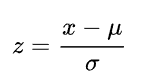
the place: μ is the imply and σ is the normal deviation of every characteristic throughout
the dataset.
Luckily, since we’re working with Python and Numpy, this may be completed by a single line of code.
# Assuming the info is saved within the numpy array F
F = (F - F.imply(axis=0)) / F.std(axis=0)
This can present the next desk:
┌────────┬───────┬───────┬───────┬───────┬───────┐
│ Pattern │  f1   │  f2   │  f3   │  f4   │  f5   │
├────────┼───────┼───────┼───────┼───────┼───────┤
│      0 │ -0.51 │ -1.14 │     0 │  1.89 │ -0.63 │
│      1 │ -0.98 │  0.01 │  0.43 │ -0.89 │ -0.02 │
│      2 │ -1.01 │ -1.14 │ -1.84 │ -1.21 │ -1.62 │
│      3 │ -1.41 │   1.4 │  0.67 │  1.79 │  1.22 │
│      4 │  0.13 │  0.99 │  0.27 │ -0.46 │ -1.19 │
│      5 │   0.7 │  -1.4 │  0.02 │  0.07 │   0.4 │
│      6 │  1.77 │  0.32 │   0.8 │  0.17 │  1.55 │
│      7 │ -0.19 │  0.28 │  1.64 │ -0.33 │ -0.46 │
│      8 │  1.45 │  1.35 │ -0.45 │ -0.67 │ -0.33 │
│      9 │  0.06 │ -0.67 │ -1.54 │ -0.37 │   1.1 │
└────────┴───────┴───────┴───────┴───────┴───────┘
Now we see that every one options are comparable to one another, in comparison with our authentic dataset.
Since we adopted the steps above, we now have a superb set of characteristic vectors. However wait! There’s something we have to do earlier than we are able to prepare our mannequin with it. We must always not use the whole dataset to coach our mannequin, as a result of we have to break up the dataset into two, or ideally three, subsets. These subsets are referred to as coaching information, validation information, and check information.
The coaching information is used to coach the mannequin.
The check information is used to judge the accuracy and efficiency of the skilled mannequin. It is crucial that the mannequin by no means sees this information throughout coaching as a result of then, we will probably be testing the mannequin on the info it has already seen.
The validation information isn’t wanted for each mannequin. Nevertheless, it could actually assist when the fashions are deep studying fashions. This dataset is used equally to how the check information is used throughout the coaching course of. It tells us how effectively the coaching course of goes and gives details about when to cease coaching and whether or not the mannequin is appropriate for the info.
In abstract, coaching and validation information are used to construct the mannequin. The check information is held again to judge the mannequin.
How a lot information ought to be put in every set?
It’s thought of normal observe to separate 90% of the set into coaching and 5% every for validation and check information in keeping with some literature, whereas others counsel 70% for coaching and 15% every for validation and check for smaller datasets or 80% for coaching and 10% for validation and check.
It is very important protect the prior possibilities within the dataset. If a category exists in real-world instances with an opportunity of 20%, this ought to be mirrored in our dataset as effectively. This must also prolong to the subsets that we create. How can we do that? There are two methods:
- Partitioning by class
- Random sampling
Partitioning by class
This methodology can be utilized when you find yourself working with small datasets. First, we decide what number of samples are current for every class. Subsequent, for every class, we put aside the chosen percentages and merge the whole lot collectively.
For instance, assume we’ve got 500 samples, with 400 belonging to class 0 and 100 from class 1. We wish to do a 90/5/5 break up (90% coaching information, 5% check, and 5% validation). This implies we randomly choose 360 samples from class 0 and 90 samples from class 1 to create the coaching set. From the remaining unused 40 samples of sophistication 0, 20 randomly chosen samples will go to validation information and 20 to check information. From the remaining unused 10 samples of sophistication 1, 5 every will go into validation and check datasets.
Random sampling
If we’ve got enough information, we don’t should be very exact and observe the above methodology. As an alternative, we are able to randomize the whole dataset and break up our information in keeping with the mandatory percentages.
However what if we’ve got a small dataset? We will use strategies equivalent to k-fold cross-validation to make sure that points with this methodology, equivalent to imbalances in prepare and check information could be mitigated. Take a look at my publish beneath if you want to study extra about this methodology.
Now, we’ve got carried out numerous operations to make sure that our information set is sufficiently good to coach a mannequin. We made certain that it has good options, that there aren’t any lacking options, and that the options are normalized. We additionally partitioned the dataset into subsets in a correct method.
The ultimate necessary step is to have one final take a look at the info to verify the whole lot is smart. This permits us to establish any mislabeled information and lacking or outlier information. These errors could be recognized by loading the info right into a spreadsheet or for bigger units, utilizing Python scripts to summarize the info. We must always take a look at values such because the imply, median, and normal deviation in addition to most and minimal values to see if there are any uncommon information. We will additionally generate boxplots to establish outliers.

After performing all of the above steps, we could be assured that our dataset is a correct dataset that may assist a mannequin prepare effectively and in flip, produce correct and dependable predictions on real-world information. It would look like numerous effort, however all the time bear in mind, in case you feed your machine studying fashions rubbish, they’ll solely output rubbish. It’s best to all the time be sure that your dataset is sufficiently ok.
On this publish, we checked out why a superb dataset is necessary. We then checked out what makes a dataset by wanting on the parts equivalent to lessons and options. We went over information preparation and find out how to deal with lacking options and scale options. Subsequent, we mentioned why and the way we should always partition the dataset. Lastly, we checked out why we should always have a closing take a look at our information and find out how to discover issues that would nonetheless exist, equivalent to outliers and mislabeled information.
