Breaking it Down: Logistic Regression | by Jacob Bumgarner | Aug, 2022

Exploring the basics of logistic regression with NumPy, TensorFlow, and the UCI Coronary heart Illness Dataset

Define:
1. What's Logistic Regression?
2. Breaking Down Logistic Regression
1. Linear Transformation
2. Sigmoid Activation
3. Cross-Entropy Loss Perform
4. Gradient Descent
5. Becoming the Mannequin
3. Studying by Instance with the UCI Coronary heart Illness Dataset
4. Coaching and Testing Our Classifier
5. Implementing Logistic Regression with TensorFlow
6. Abstract
7. Notes and Sources

Logistic regression is a supervised machine studying algorithm that creates classification labels for units of enter knowledge (1, 2). Logistic regression (logit) fashions are utilized in quite a lot of contexts, together with healthcare, analysis, and enterprise analytics.

Understanding the logic behind logistic regression can present sturdy foundational perception into the fundamentals of deep studying.

On this article, we’ll break down logistic regression to realize a elementary understanding of the idea. To do that, we are going to:

1. Discover the elemental elements of logistic regression and construct a mannequin from scratch with NumPy
2. Practice our mannequin on the UCI Coronary heart Illness Dataset to foretell whether or not adults have coronary heart illness primarily based on their enter well being knowledge
3. Construct a ‘formal’ logit mannequin with TensorFlow

You may observe the code on this publish with my walkthrough Jupyter Pocket book and Python script recordsdata in my GitHub learning-repo.

Logistic regression fashions create probabilistic labels for units of enter knowledge. These labels are sometimes binary (sure/no).

Let’s work by an instance to spotlight the foremost points of logistic regression, after which we’ll begin our deep dive:

Think about that we’ve got a logit mannequin that’s been skilled to foretell if somebody has diabetes. The enter knowledge to the mannequin are an individual’s age, peak, weight, and blood glucose. To make its prediction, the mannequin will remodel these enter knowledge utilizing the logistic perform. The output of this perform will likely be a probabilistic label between 0 and 1. The nearer this label is to 1, the larger the mannequin’s confidence that the particular person has diabetes, and vice versa.

Importantly: to create classification labels, our diabetes logit mannequin first needed to be taught the right way to weigh the significance of every piece of enter knowledge. It’s possible that somebody’s blood glucose must be weighted greater than their peak for predicting diabetes. This studying occurred utilizing a set of labeled check knowledge and gradient descent. The realized data is saved within the mannequin within the type of Weights and bias parameter values used within the logistic perform.

This instance supplied a satellite-view define of what logistic regression fashions do and the way they work. We’re now prepared for our deep dive.

To begin our deep dive, let’s break down the core part of logistic regression: the logistic perform.

Relatively than simply studying from studying alone, we’ll construct our personal logit mannequin from scratch with NumPy. This would be the mannequin’s define:

In sections 2.1 and 2.2, we’ll implement the linear and sigmoid transformation features.

In 2.3 we’ll outline the cross-entropy price perform to inform the mannequin when its predictions are ‘good’ and ‘dangerous’. In part 2.4 we’ll assist the mannequin be taught its parameters by way of gradient descent.

Lastly, in part 2.5, we’ll tie all of those features collectively.

2.1 Linear Transformation

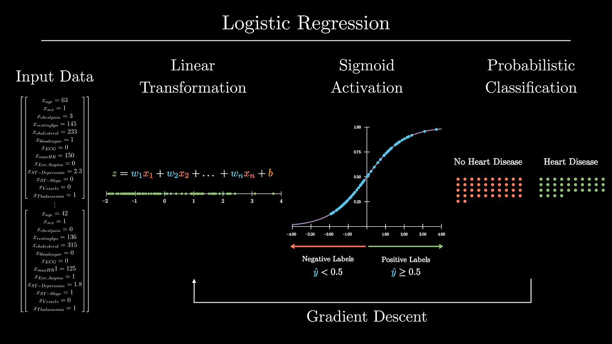
As we noticed above, the logistic perform first applies a linear transformation to the enter knowledge utilizing its realized parameters: the Weights and bias.

The Weights (W) parameters point out how essential each bit of enter knowledge is to the classification. The nearer a person weight is to 0, the much less essential the corresponding piece of information is to the classification. The dot product of the Weights vector and enter knowledge X flattens the info right into a single scalar that we will place onto a quantity line.

For instance, if we’re making an attempt to foretell whether or not somebody is drained primarily based on their peak and the hours they’ve spent awake, the burden for that particular person’s peak can be very near zero.

The bias (b) parameter is used to shift this scalar alongside the choice boundary of this line (0).

Let’s visualize how the linear part of the logistic perform makes use of its realized weights and bias to rework enter knowledge from the UCI Coronary heart Illness Dataset.

We’re now prepared to begin populating our mannequin’s features. To begin, we have to initialize our mannequin with its Weights and bias parameters. The Weights parameter will likely be an (n, 1) formed array, the place n is the same as the variety of options within the enter knowledge. The bias parameter is a scalar. Each parameters will likely be initialized to 0.

Subsequent, we will populate the perform to compute the linear portion of the logistic perform.

2.2 Sigmoid Activation

Logistic fashions create probabilistic labels (ŷ) by making use of the sigmoid perform to the output knowledge from the logistic perform’s linear transformation. The sigmoid perform is beneficial to create possibilities from enter knowledge as a result of it squishes enter knowledge to provide values between 0 and 1.

The sigmoid perform is the inverse of the logit perform, therefore the identify, logistic regression.

To create binary labels from the output of the sigmoid perform, we outline our determination boundary to be 0.5. Which means if ŷ ≥ 0.5, we are saying the label is optimistic, and when ŷ < 0.5, we are saying the label is destructive.

Let’s visualize how the sigmoid perform transforms the enter knowledge from the linear part of the logistic perform.

Now, let’s implement this perform into our mannequin.

2.3 Cross-Entropy Price Perform

To show our mannequin the right way to optimize its Weights and bias parameters, we are going to feed in coaching knowledge. Nonetheless, for the mannequin to be taught optimum parameters, it should know the right way to inform if its parameters did a ‘good’ or ‘dangerous’ job at producing probabilistic labels.

This ‘goodness’ issue, or the distinction between the chance label and the ground-truth label, is known as the loss for particular person samples. We operationally say that losses must be excessive if the parameters did a nasty job at predicting the label and low in the event that they did an excellent job.

The losses throughout the coaching knowledge are then averaged to create a price.

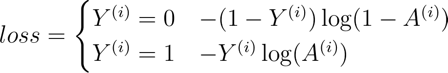
The perform that has been adopted for logistic regression is the Cross-Entropy Price Perform. Within the perform under, Y is the ground-truth label, and A is our probabilistic label.

Discover that the perform modifications primarily based on whether or not y is 1 or 0.

• When y = 1, the perform computes the log of the label. If the prediction is right, the loss will likely be 0 (i.e., log(1) = 0). If it’s incorrect, the loss will get bigger and bigger because the prediction approaches 0.
• When y = 0, the perform subtracts 1 from y after which computes the log of the label. This subtraction retains the loss low for proper predictions and excessive for incorrect predictions.

Let’s now populate our perform to compute the cross-entropy price for an enter knowledge array.

2.4 Gradient Descent

Now that we will compute the price of the mannequin, we should use the price to ‘tune’ the mannequin’s parameters by way of gradient descent. If you happen to want a refresher on gradient descent, take a look at my Breaking it Down: Gradient Descent publish.

Let’s create a pretend situation: think about that we’re coaching a mannequin to foretell if an grownup is drained. Our pretend mannequin solely will get two enter options: peak and hours spent awake. To precisely predict if an grownup is drained, the mannequin ought to most likely develop a really small weight for the peak characteristic, and a a lot bigger weight for the hours spent awake characteristic.

Gradient descent will step these parameters down their gradient such that their new values will produce smaller prices. Keep in mind, gradient descent minimizes the output of a perform. We will visualize our imaginary instance under.

To compute the gradient of the price perform w.r.t. the Weights and the bias, we’ll should implement the chain rule. To search out the gradients of our parameters, we’ll differentiate the price perform and the sigmoid perform to seek out their product. We’ll then differentiate the linear perform w.r.t the Weights and bias perform individually.

Let’s discover a visible proof of the partial differentiations for logistic regression:

Let’s implement these simplified equations to compute the common gradients for every parameter throughout the coaching examples.

Lastly, we’ve constructed all the mandatory elements for our mannequin, so now we have to combine them. We’ll create a perform that’s suitable with each batch and mini-batch gradient descent.

• In batch gradient descent, each coaching pattern is used to replace the mannequin’s parameters.
• In mini-batch gradient descent, a random portion of the coaching samples is chosen to replace the parameters. Mini-batch choice isn’t that essential right here, however it’s extraordinarily helpful when coaching knowledge are too massive to suit into the GPU/RAM.

As a reminder, becoming the mannequin is a three-step iterative course of:

1. Apply linear transformation to enter knowledge with the Weights and Bias
2. Apply non-linear sigmoid transformation to accumulate a probabilistic label.
3. Compute the gradients of the price perform w.r.t W and b and step these parameters down their gradients.

Let’s construct the perform!

To verify we’re not simply making a mannequin in isolation, let’s prepare the mannequin with an instance human dataset. Within the context of scientific well being, the mannequin we’ll prepare may enhance doctor consciousness of affected person well being dangers.

Let’s be taught by instance with the UCI Coronary heart Illness Dataset.

The dataset accommodates 13 options in regards to the cardiac and bodily well being of grownup sufferers. Every pattern can also be labeled to point whether or not the topic does or doesn’t have coronary heart illness.

To begin, we’ll load the dataset, examine it for lacking knowledge, and study our characteristic columns. Importantly, the labels are reversed on this dataset (i.e., 1=no illness, 0=illness) so we’ll have to repair that.

Variety of topics: 303
Share of topics identified with coronary heart illness:  45.54%
Variety of NaN values within the dataset: 0

Let’s additionally visualize the options. I’ve created customized figures, however see my gist right here to create your personal with Seaborn.

From our inspection, we will conclude that there are not any apparent lacking options. We will additionally see that there are some stark group separations in a number of of the options, together with age (age), exercise-induced angina (exang), chest ache (cp), and ECG shapes throughout train (oldpeak & slope). These knowledge will likely be good to coach a logit mannequin!

To conclude this part, we’ll end getting ready the dataset. First, we’ll do a 75/25 cut up on the info to create check and prepare units. Then we’ll standardize* the continual options listed under.

to_standardize = ["age", "trestbps", "chol", "thalach", "oldpeak"]

*You don’t should standardize knowledge for logit fashions until you’re working some type of regularization. I do it right here simply as a greatest apply.

4. Coaching and Testing Our Classifier

Now that we’ve constructed the mannequin and ready our dataset, let’s prepare our mannequin to foretell well being labels.

We’ll instantiate the mannequin, prepare it with our x_train and y_train knowledge, and we’ll check it with the x_test and y_test knowledge.

Remaining mannequin price: 0.36
Mannequin check prediction accuracy: 86.84%

And there we’ve got it: a check set accuracy of 86.8%. That is significantly better than a 50% random likelihood, and for such a easy mannequin, the accuracy is kind of excessive.

To examine issues a bit extra intently, let’s visualize the mannequin’s options throughout its coaching. On the highest row, we will see the mannequin’s price and accuracy throughout its coaching. Then on the underside row, we will see how the Weights and bias parameters change throughout coaching (my favourite half!).

5. Implementing Logistic Regression with TensorFlow

In the true world, it’s not greatest apply to construct your personal mannequin when you have to use one. As a substitute, we will depend on highly effective and well-designed open-source packages like TensorFlow, PyTorch, or scikit-learn for our ML/DL wants.

Beneath, let’s see how easy it’s to construct a logit mannequin with TensorFlow and examine its coaching/check outcomes to our personal. We’ll put together the info, create a single-layer and single-unit mannequin with a sigmoid activation, and we’ll compile it with a binary cross-entropy loss perform. Lastly, we’ll match and consider the mannequin.

Epoch 5000/5000
1/1 [==============================] - 0s 3ms/step - loss: 0.3464 - accuracy: 0.8634Check Set Accuracy:
1/1 [==============================] - 0s 191ms/step - loss: 0.3788 - accuracy: 0.8553
[0.3788422644138336, 0.8552631735801697]

From this, we will see that the mannequin’s closing coaching price was 0.34 (in comparison with our 0.36), and the check set accuracy was 85.5%, similar to our consequence above. There are a couple of minor variations below the hood, however the mannequin performances are very related.

Importantly, the TensorFlow mannequin was constructed, skilled, and examined in lower than 25 strains of code, versus our 200+ strains of code within thelogit_model.py script.

On this publish, we’ve explored all the particular person points of the logistic regression. We began the publish by constructing a mannequin from scratch with NumPy. We first carried out the linear and sigmoid transformations, carried out the binary-cross entropy loss perform, and created a becoming perform to coach our mannequin with enter knowledge.

To know the aim of logistic regression, we then coaching our NumPy mannequin on the UCI Coronary heart Illness Dataset to foretell coronary heart illness in sufferers. We discovered noticed the straightforward mannequin had an 86% prediction accuracy — fairly spectacular.

Lastly, after taking the time to be taught and perceive these fundamentals, we then noticed how straightforward it was to construct a logit mannequin with TensorFlow.

In sum, logistic regression is each a helpful algorithm for predictive evaluation. Understanding this mannequin is a strong first step within the highway of learning deep studying.