A step-by-step information to analysing Strava information with Python
A few years in the past I taught myself how you can use R by analysing my Strava information. It was a enjoyable technique to study and mixed two of my passions – information and operating (effectively, sport basically).
Now, I’m doing the identical in Python. On this publish I’ll be sharing the steps I took in performing some information wrangling and Exploratory Information Evaluation (EDA) of my Strava information, while hopefully pulling out some fascinating insights and sharing helpful suggestions for different Python newbies. I’m comparatively new to Python however I discover that documenting the method helps me study and may allow you to too!
Downloading your Strava information
First off, we have to get our dataset. I downloaded my information as a CSV from the Strava web site, however you may as well join on to the Strava API.
To get your information from the Strava web site, navigate to your profile by clicking your icon on the highest proper hand facet of the web page. Navigate to ‘My Account’ and hit ‘Get Began’ on the backside of the web page.

On the subsequent web page you’ll see three choices. Beneath choice 2 ‘Obtain Request’, hit ‘Request Your Archive’. Shortly after (often below an hour relying on the dimensions of the archive) the e-mail related together with your Strava account will obtain your archive in a zipper file format. The file you need might be referred to as actions.csv, I are inclined to ignore the remainder of the information in there.
Navigate to your Jupyter Pocket book and add the CSV by hitting the add information button, beneath ‘View’.

You must now see your CSV within the file browser, on the left hand facet of your Jupyter pocket book.
Import Libraries
Now we have to obtain the libraries we’ll be utilizing for the evaluation.
import pandas as pd
import matplotlib.pyplot as plt
import numpy as np
import seaborn as sns
from datetime import datetime as dt
Subsequent we have to remodel the CSV we’ve uploaded into Jupyter right into a desk format utilizing the Pandas library, which is a really highly effective and in style framework for information evaluation and manipulation.
df = pd.read_csv('strava_oct_22.csv') #learn in csv
df.columns=df.columns.str.decrease() #change columns to decrease case
Information Wrangling
I do know from previous expertise that the actions obtain from Strava features a entire host of nonsensical and irrelevant fields. Due to this fact, I need to cleanse the dataset somewhat earlier than getting caught in.
Beneath are a few capabilities which allow you to get a really feel to your dataset:
df.form(818, 84)
The form perform tells you the variety of rows and columns inside your dataset. I can see I’ve 818 rows of information (every row is exclusive to a person exercise) and 84 columns (also referred to as variables or options). I do know the vast majority of these columns might be ineffective to me as they’re both NaN values (Not a Quantity) or simply not helpful, however to verify we will use the .head() perform, which brings again the highest 5 values for every column inside the dataset.

We will additionally use .information() to convey again all of the column titles for the variables inside the dataset.

You may as well see the ‘ Non Null Counts’ beneath every variable within the output above, which provides you an thought of what number of rows for that variable are populated. Let’s eliminate the pointless noise by deciding on solely columns that we predict might be related.
#Create new dataframe with solely columns I care about
cols = ['activity id', 'activity date', 'activity type', 'elapsed time', 'moving time', 'distance',
'max heart rate', 'elevation gain', 'max speed', 'calories'
]
df = df[cols]
df
That appears higher, however the dataset is lacking some key variables that I need to embrace in my evaluation which aren’t a part of the extract by default, for instance common tempo and km per hour. Due to this fact, I must compute them myself. Earlier than I try this I must double test the datatypes in my new information body to make sure that every area is within the format I want it to be in. We will use .dtypes to do that.
df.dtypes

I can see that almost all of the fields within the dataset are numeric (int64 is a numeric worth as is float64, however with decimals). Nonetheless I can see that the exercise date is an object which I might want to convert to a date datatype after I come to have a look at time sequence evaluation. Equally, distance is an object, which I must convert to a numeric worth.
I can use the datetime library to transform my exercise date from object to a date datatype. We will additionally create some extra variables from exercise date, i.e. pulling out the month, yr and time, which we are going to use later within the evaluation.
#Break date into begin time and date
df['activity_date'] = pd.to_datetime(df['activity date'])
df['start_time'] = df['activity_date'].dt.time
df['start_date_local'] = df['activity_date'].dt.date
df['month'] = df['activity_date'].dt.month_name()
df['year'] = df['activity_date'].dt.yr
df['year'] = (df['year']).astype(np.object) #change yr from numeric to object
df['dayofyear'] = df['activity_date'].dt.dayofyear
df['dayofyear'] = pd.to_numeric(df['dayofyear'])
df.head(3)
Subsequent we have to convert distance to be a numeric worth utilizing the to_numeric perform from the Pandas library. It will enable us to successfully create our new variables wanted for the evaluation.
#convert distance from object to numeric
df['distance'] = pd.to_numeric(df['distance'], errors = 'coerce')
Now that distance is a numeric worth, I can create some extra variables to incorporate in my information body.
#Create additional columns to create metrics which are not within the dataset already
df['elapsed minutes'] = df['elapsed time'] /60
df['km per hour'] = df['distance'] / (df['elapsed minutes'] / 60)
df['avg pace'] = df['elapsed minutes'] / df['distance']
Since I’ve added and amended some variables, let’s use .dtypes once more to test the info body is in the fitting format.

That appears significantly better. Lastly, earlier than we transfer onto the EDA I would like my dataset to incorporate runs solely, as I do know that almost all of my actions are of this kind. To substantiate I can rely the variety of actions for every exercise sort utilizing .value_counts().
df['activity type'].value_counts()

As you possibly can see, the overwhelming majority of my actions are runs, so I’m going to make a brand new information body referred to as ‘runs’ and focus solely on that. I additionally know that there’s a couple of inaccurate information entries within the information, the place I’ll have forgotten to cease my watch or Strava was having a meltdown, so I’m additionally going to filter out some excessive outcomes.
runs = df.loc[df['activity type'] == 'Run']
runs = runs.loc[runs['distance'] <= 500]
runs = runs.loc[runs['elevation gain'] <= 750]
runs = runs.loc[runs['elapsed minutes'] <= 300]
runs = runs.loc[runs['year'] >= 2018]
Exploratory Information Evaluation
We now have a cleansed dataset that we will begin to visualise and pull out fascinating insights from. A great first step in EDA is to create a pairs plot, which shortly lets you see each distribution of single variables and relationships between two variables. It is a nice methodology to establish traits for follow-up evaluation. You probably have numerous variables in your dataset this may get messy, so I’m going to select a couple of to give attention to.
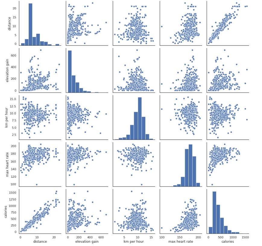
pp_df = runs[['distance', 'elevation gain', 'km per hour', 'max heart rate', 'calories']]
sns.pairplot(pp_df);

That one line of code is fairly highly effective and we will already pull out some helpful insights from this. The histograms on the diagonal permits us to see the distribution of a single variable while the scatter plots on the higher and decrease triangles present the connection (or lack thereof) between two variables. I can see that there’s a optimistic correlation between distance and energy. I can see on the space histogram that there’s a left skew, that means extra of my runs are of a shorter distance. It’s additionally fascinating that energy comply with an inverse skew to km per hour and max coronary heart fee — Pushing your self more durable doesn’t essentially imply extra energy misplaced.
The pairs plot is a pleasant technique to visualise your information, however you may need to have a look at some abstract statistics of your dataset, to get an thought of the imply, median, normal deviation and many others. To do that, use the .describe perform.
runs.describe().spherical(0)

I actually just like the describe perform, it’s a fast technique to get a abstract of your information. My first response after I noticed the above output was shock that for distance, the median (or fiftieth percentile) of my runs is simply 6km! However then once more, I feel I’ve ramped up my distance solely within the final yr or so. The fantastic thing about EDA is that as you’re performing preliminary investigations on information, you’ll be able to uncover patterns, spot anomalies, check speculation and test assumptions, so let’s see dig somewhat deeper into the space variable.
I’m going to visualise the unfold of the space by yr utilizing a boxplot, to see if my speculation that I’ve elevated my distance within the final yr is right. A boxplot is a good way of exhibiting a visible abstract of the info, enabling us to establish imply values, the dispersion of the dataset, and indicators of skewness.

fig, ax = plt.subplots()
sns.set(model="whitegrid", font_scale=1)
sns.boxplot(x="yr", y="distance", hue="yr", information=runs)
ax.legend_.take away()
plt.gcf().set_size_inches(9, 6)
As I assumed, my runs have certainly elevated in distance within the final couple of years, with the median distance growing barely annually from 2018 till 2022 when it elevated rather more significantly.
Let’s breakout the years by month to see how distance coated varies all through yr. We will do that through the use of a bar plot from the seaborn library.
sns.set_style('white')
sns.barplot(x='month', y='distance', information=runs, hue='yr', ci=None, estimator=np.sum, palette = 'scorching',
order =["January", "February", "March", "April", "May", "June", "July", "August", "September", "October", "November", "December"])
plt.gcf().set_size_inches(17, 6)
plt.legend(loc='higher heart')
#plt.legend(bbox_to_anchor=(1.05, 1), loc='higher proper', borderaxespad=0)
;

It’s clear from the above bar plot is that my distance drops in the summertime months. Taking 2022 for example, in January, February and March 2022 the space I ran was over 150km, notably greater than what I cowl in April-August. This pattern is clear in different years too.
Let’s create a brand new variable referred to as season by grouping months into their respective season utilizing .isin().
runs['season'] = 'unknown'
runs.loc[(runs["month"].isin(["March", "April", "May"])), 'season'] = 'Spring'
runs.loc[(runs["month"].isin(["June", "July", "August"])), 'season'] = 'Summer time'
runs.loc[(runs["month"].isin(["September", "October", "November"])), 'season'] = 'Autumn'
runs.loc[(runs["month"].isin(["December", "January", "February"])), 'season'] = 'Winter'
We will now create one other boxplot to visualise distance by season.
ax = sns.boxplot(x="season", y="distance", palette="Set2",
information=runs,
order =["Spring", 'Summer', 'Autumn', 'Winter'])
plt.gcf().set_size_inches(9, 7)

For these not accustomed to boxplots, the daring line represents the median, the field represents the interquartile vary (the center 50% of the info), the decrease and higher traces characterize the min and max, and the black dots characterize outliers. I discover it actually fascinating to see how my behaviour modifications by season, it seems that I actually am not a fan of lengthy summer time runs, with 75% of my runs being below 7k.
Finish Notes
We’ve coated fairly a bit on this introduction to Python, together with how you can get began with studying a file into pandas, cleansing the dataset to optimise efficiency and creating extra variables to incorporate in our evaluation. We’ve generated some abstract statistics to raised perceive our information, and began to visualise our dataset utilizing matplotlib and seaborn.
Now the dataset is cleansed and now we have a greater understanding I’m wanting ahead to conducting additional evaluation on the info and bringing in some information science strategies. For instance, I plan to construct a linear regression mannequin to foretell what my subsequent 5k time might be, relying on variables comparable to what day/season/time of day it’s, or what the elevation of the route is, and even the temperature and wind velocity if I embrace some climate information.
Thanks for studying, till the subsequent one!

