
Continuity of likelihood measure, Radon-Nikodym spinoff, and Girsanov theorem

The Girsanov theorem and Radon-Nikodym theorem are steadily utilized in monetary arithmetic for the pricing of economic derivatives. And they’re deeply associated. The utilization of these theorems will also be present in machine studying (very theoretical although). An instance is given in [9], the place Girsanov’s concept is utilized in a brand new coverage gradient algorithm for reinforcement studying.
Nonetheless, these theorems are removed from intuitive (even the notation). Due to this fact, this submit makes an attempt to supply a transparent rationalization to them, which may be very tough to seek out. To know them correctly, we have to perceive several types of continuity of likelihood distribution first, that’s why this matter can also be included and takes a big a part of this submit.
Additionally, notice that this submit is a continuation of this, issues like filtration, martingale, Itô processes, and so forth. are already mentioned there. So if one thing will not be clear, you may check with that submit, or different two posts of mine about measure concept and concept of likelihood, or go away me a notice.
Random variables and distribution
The random variable is a really fundamental idea within the concept of likelihood and additionally it is elementary for understanding the stochastic processes. The random variable is barely talked about in my different posts about measure concept and likelihood, however right here we’ll take a look at it extra rigorously. Firstly, we present the formal definition of the random variable within the context of measure concept:
Given a likelihood triple (Ω, 𝓕, P), a random variable is a operate X from Ω to the true numbers ℝ, such that

We will see that ω is the picture of X and Situation 1.1 is similar as saying X⁻¹((-∞, x]) ∈ 𝓕. Additionally, we all know that if set A ={(-∞, x]; x ∈ ℝ}, then σ(A) = 𝓑, the place 𝓑 is the Borel σ-algebra. (This may be proved simply by proving that σ(A) accommodates all of the intervals utilizing the properties of σ-algebra.) Due to this fact, Situation 1.1 can also be the identical as X⁻¹(B) ∈ 𝓕, for all B ∈ 𝓑. [1]
The distribution of a random variable on a likelihood triple (Ω, 𝓕, P) is P (recall that it’s a operate outlined on ), the measure of the likelihood area. The distribution is outlined by (or in different phrases, the likelihood is outlined by way of a random variable by)

Word that generally you can even see the time period “likelihood regulation” or “regulation” of a random variable, however they’re the identical factor.
Continuity
We already know {that a} random variable or a distribution may be discrete, steady, or a mixture of each. However there may be nonetheless one thing lacking, and on this part, we’ll assessment what we already knew and fill the hole.
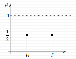
(1) discrete: a likelihood measure μ is discrete if all of its mass is at every particular person level. The only instance is a coin toss, whose graph is proven under:
(2) completely steady: this property can check with each random variable and measure and is outlined in another way. Nonetheless, they’re intrinsically related, so each of them will likely be mentioned right here and it’s important at all times to bear in mind the connection between a likelihood measure and a random variable.
a. Firstly we take a look at the case of measure. It’s outlined with regard to a different measure, which serves as a reference. We are saying that ν is completely steady with respect to μ, if ν(A) = 0 for any A ∈ 𝓑 such that μ(A) = 0. This relationship between ν and μ is often denoted by ν ≪ μ. [2] We will additionally say that μ dominates ν. If it applies that each ν ≪ μ and μ ≪ ν, then we are saying that these two measures are equal, which is often denoted as ν ~ μ. Extra intuitively, we are able to consider ν as a extra “delicate” measure, if μ tells us that the measure of a set is zero, then ν won’t output a bigger consequence.
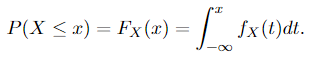
b. Within the case of a random variable, a random variable X: Ω → ℝ is completely steady if there exists an integrable non-negative operate fₓ: ℝ → ℝ⁺ (that is the likelihood density operate) such that for all x ∈ ℝ,
Typically we are able to additionally see that fₓ is integrable over all any Borel units (components in 𝓑), based on what we now have mentioned in part random variables, these two variations of the definition are the identical.
Two questions come up: 1. what’s the connection between “continuity” and “absolute continuity”? 2. What does continuity should do with measure? (now we’re solely speaking about random variables)
Firstly we’ll reply the second query: as mentioned right here, if P(X = x) = 0, for all of the x ∈ ℝ, then X is a steady variable. (Intuitively, when the random variable is steady, it may possibly take any worth on the true line, and on this case, the measure provides us the “size of a degree”). Now we take a look at the primary query: From the definition of absolute continuity and we are able to derive
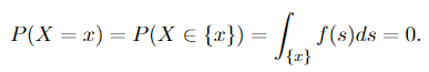
It’s apparent why Equation 1.3 applies: the combination over a singleton set is zero. Since we now have P(X = x) = 0 for all of the x ∈ ℝ, as mentioned above, X is steady. Due to this fact, we now have the assertion:
Any completely steady random variable can also be steady.
And the next truth builds the bridge between absolute continuity and measure:
A random variable is completely steady if and provided that each set of measure zero has zero likelihood.
(3) singularly steady: right here once more, we now have “singular steady measure” and “singularly steady distribution”, and once more they’re related. And really even nearer to one another than within the earlier case (continuity). We’ll take a look at the definitions of each of these ideas first after which give a concrete instance. It’s a matter, which is seldom included within the undergraduate examine materials. However after we get to know this, all of the varieties of likelihood distributions are lined.
It isn’t essential to undergo the main points of singular continuity in the event you simply wish to perceive the Girsanov theorem, for which moderately the “absolute continuity” is vital. Nonetheless, I imagine it’s useful to be taught the speculation of likelihood, to know all these varieties of distribution.
a. A singularly steady distribution on ℝⁿ is a likelihood distribution focused on a set of Lebesgue measure zero, however the measure of each level on this set can also be zero.
b. And a measure μ is singularly steady with regard to measure λ if μ{x} = 0 for all x ∈ ℝ, however there may be S ⊆ ℝ with λ(S) = 0 and μ(Sᶜ) = 0, which implies μ(S) = 1. One other identify, singular measure, will also be encountered and might seem to have barely totally different definitions, however right here for simplicity and readability, we use the model in [1] and can keep away from the time period “singular measure”.
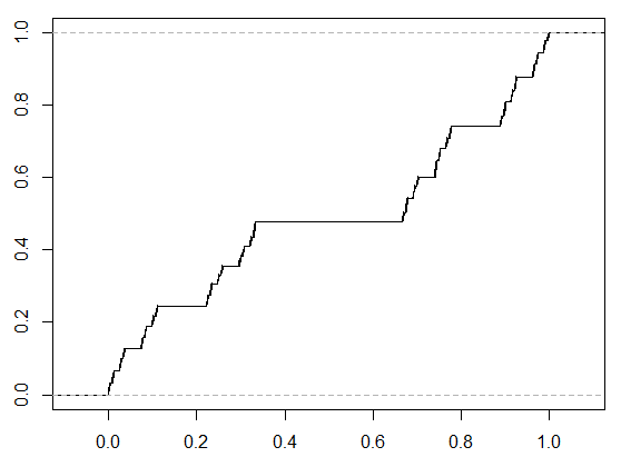
Some examples may be helpful for understanding singular continuity. Within the one-dimensional case (one random variable is concerned), an instance is Cantor’s operate. As a consequence of its form, additionally it is known as the “satan’s staircase”. (see Determine 1.4) Such a cumulative distribution operate (CDF) is steady however has zero derivatives nearly (we now have seen this phrase earlier than) all over the place. The weird factor is that it’s not rising based on the spinoff, however it’s certainly growing by building.
Much less pathological examples exist in greater dimensions (Take into consideration this: we wish to assemble a set with Lebesgue measure zero, and within the set, each level will even have measure zero — naturally, this will likely be one thing like “the world of a line” or “the amount of a aircraft”, which can’t be present in one-dimensional area.), the place the joint distribution of a number of random variables will likely be thought of. Right here we’ll present an instance with two random variables taken from [4]:
There are two gadgets, which generate a random quantity from 0 to 1. Nonetheless, one in every of them is damaged and at all times provides 0. A statistician makes use of one in every of them every day, for 2 steady days. He chooses randomly from these two gadgets (in fact, it’s attainable that he makes use of the identical gadget for each days). Let X signify the quantity acquired on the primary day and Y denote the quantity acquired on the second day. What’s the joint distribution of X and Y?
We will simply see that this distribution is neither completely steady nor discrete because the distribution of the output of the nice gadget is uniform however that of the damaged one is discrete. To investigate what it truly is, we will even discuss concerning the decomposition of likelihood distribution by way of this instance.
For a extra intuitive understanding, right here I provide a crappy scratch of the distribution operate:
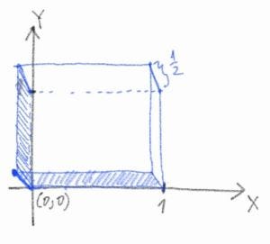
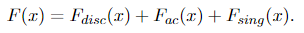
Word that f(0, 0) = 1/2, which implies that half of the mass is focused on the purpose (0, 0). It corresponds to the occasion that on each days, the statistician will get output zero. And the opposite half of the mass is evenly unfold on the one-by-one unit sq. (the amount is 1 × 1 × 1/2 = 1/2). We will additionally discover the singular part within the CDF. With out lack of generality, we attempt to determine the cumulative distribution of X first. In line with Lebesgue’s decomposition theorem, any likelihood measure μ may be decomposed as

Because the CDF uniquely determines the distribution of a random variable (consider the definition), we are able to additionally decompose the CDF into the shape given by Equation 1.6, particularly
The CDF of X doesn’t have any singular half. And each discrete half and absolute steady half may be simply decided:
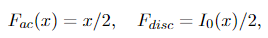
the place Iᵣ(x) denotes the next operate

Due to this fact, we now have
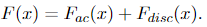
and based on the unbiased similar distribution (i.i.d.) assumption we talked about earlier than, Y has the very same CDF as X, given by Equation 1.10. Additionally, as a result of i.i.d assumption, the CDF of X and Y is just F(x, y) = F(x)F(y), which provides us
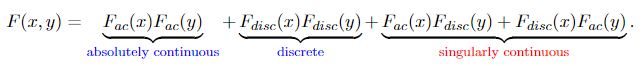
The joint CDF of X and Y have all three components as anticipated. The singularly steady half corresponds to the occasion that one of many gadgets is damaged and one other is nice, which corresponds to the shaded space within the graph of the joint likelihood density operate of X and Y given in Determine 1.5 — they’ve Lebesgue measure zero in three-dimensional area, and the measure outlined on this area comparable to the singular steady half in Equation 1.11. However on this space, the measure of every level is zero.
Now we glance again on the definition of singularly steady measure, clearly, we are able to name the measure on the shaded space μ₁ (on condition that one of many gadgets is damaged — a sub-sample area), and one other μ₂ within the 3d area (the unique pattern area), we are able to see simply that μ₁ is singular with regard to μ₂.
Radon-Nikodym spinoff
The Radon-Nikodym spinoff is, in truth, a ratio of two measures, which has nothing to do with the “spinoff” in actual evaluation, within the sense that the spinoff in actual evaluation describes how briskly a operate modifications, however the Radon-Nikodym spinoff is nothing like this. Nonetheless, they do have some similarities. We will see this from the next properties of the Radon-Nikodym spinoff: Let ν be a σ-finite measure on a measure area (Ω, 𝓕) [7], (ν is σ-finite implies that Ω is a countable union of units with finite measures)
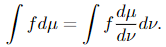
(1) if μ is a measure, μ ≪ ν and f ≥ 0 is a μ-integrable operate, then
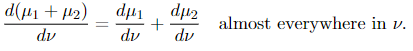
(2) If μᵢ, i= 1, 2 are measures and μᵢ ≪ ν, then μ₁ + μ₂ ≪ ν and
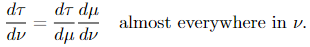
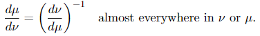
(3) (Chain rule) If 𝜏 is a measure, μ is a σ-finite measure, and 𝜏 ≪ μ ≪ ν, then
If μ and ν are equal, then
The Radon-Nikodym throrem
The Radon-Nikodym theorem exhibits a approach to categorical one measure by way of one other measure by way of some linear operator. And on this case, the illustration is by way of the integral operator (the integrator — this time period is used right here). The Radon-Nikodym theorem says
Given a measurable area (Ω, 𝓕), if a σ-finite measure ν on (Ω, 𝓕) is completely steady with respect to a σ-finite measure μ on (Ω, 𝓕), then there’s a non-negative measurable operate f on Ω such that
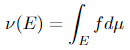
for any measurable set E.
Why is that this theorem vital? One factor is that it may be used to point out the existence of conditional expectation. Earlier than we present the definition of the conditional expectation, we want to pay attention to the truth that the conditional expectation of random variable X, given the σ-algebra 𝓕, denoted by E[X | 𝓕], is itself a (𝓕-measurable) random variable. The definition is given as follows:
We name a random variable Y to the conditional expectation of X, i.e. Y = E[X | 𝓕]. Two situations should be happy
(1) Y is 𝓕-measurable.
(2) For all A ∈ 𝓕, we now have
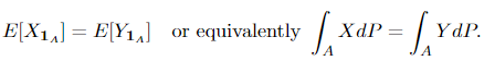
1_A denotes the character (indicator) operate. Extra intuitively, which means given data 𝓕 (check with this to see why it’s referred to as “data” and what it means), Y is the perfect prediction of X. And the next theorem, which may be proved utilizing the Radon-Nikodym theorem, exhibits the existence and uniqueness of the conditional expectation:
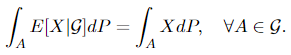
Take into account a likelihood area (Ω, 𝓕, P), a random variable X on it, and a sub-σ-algebra 𝓖 ⊆ 𝓕. If E[X] is well-defined, then there exists a 𝓖-measurable operate E[X|𝓖] distinctive to P-null units (the measure P provides zero on these units), such that
An important purpose why we point out the Radon-Nikodym theorem in that is that it’s intently associated to the change of measure, which is key within the Girsanov theorem. Now we current the next theorem:
If P and Q are equal likelihood measures, and X(t) is an 𝓕ₜ-adapted course of, let dQ/dP be the Radon-Nikodym spinoff and L(s) = Eₚ[dQ/dP|𝓕ₛ], then for s < t
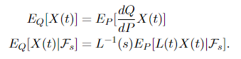
The second equality is sort of technical to show, so it’s not included right here, however the first one is tremendous straightforward to point out utilizing property (1) of the Radon-Nikodym spinoff:
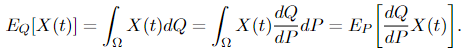
And the Radon-Nikodym theorem ensures that the Radon-Nikodym spinoff dQ/dP exists, which is also called the density of X.
Firstly, we briefly introduce what’s Wiener measure as a result of under we will likely be speaking about Wiener processed and Wiener processes with drifts. The Wiener measure is the measure outlined on Wiener area, which is the area C[0, 1] of steady real-valued capabilities x on the interval [0, 1]. We will make a measurable area out of this, by equipping it with a σ-algebra and measure. And the Wiener measure is the distinctive measure on this area, which assigns a likelihood to each finite path. [5] Intuitively, the Wiener measure of a set is the likelihood {that a} Wiener course of trajectory is a member of that set.
The Girsanov theorem states how a stochastic course of change with the change of measure. To be extra exact, it relates a Wiener measure P to a unique measure Q on the area of steady paths by giving an specific components for the probability ratios, which is the Radon-Nikodym spinoff, between them. It additionally wants to use that P and Q are equal, which is mentioned in Part Continuity. And a bit extra perception:
The Girsanov theorem says {that a} new course of with a unique drift may be constructed from a course of with an equal measure — change within the drift of a stochastic course of doesn’t lead to dramatic change in measure. And actually, how the measure modifications, may be calculated explictely.
A barely totally different model of the Girsanov theorem states {that a} new illustration may be discovered for a stochastic course of, which has a unique drift and measure.
There’s additionally a converse model of the Girsanov theorem, which states that if we now have a course of X(t) with measure P, and one other course of Y(t) with measure Q, the place Q ~ P. Then X(t) and Y(t) may be expressed by way of one another with a drift change. We’ll introduce all three of those variations on this part. [6]
The Girsanov theorem I
Let W(t) be a Wiener course of on the filtered likelihood area
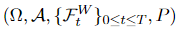
and let Y(t) ∈ ℝⁿ be an n-dimensional Itô course of of the shape

the place T ≤ ∞ is a continuing and W(t) is an n-dimensional Wiener course of. Let measure
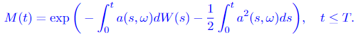
Assume that a(s, ω) satisfies Novikov’s situation, which is a ample situation for course of M(t) to be a martingale:
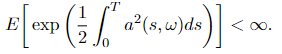
the place E = Eₚ is the expectation with regard to P. Outline the measure Q on the likelihood area of Y(t), (Ω, 𝓕_T), by
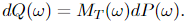
Then Y(t) is an n-dimensional Wiener course of with regard to the likelihood measure Q, for t ≤ T.
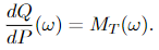
On this theorem, the Y(t) is the brand new course of after a shift within the drift of a Wiener course of. We will see that the a(t, ω) is the drift, which modifications in time. The measure of Y(t) is given by reworking the unique measure (the Wiener measure) P by way of the method Girsanov transformation given in Equation 3.2. And M(t), given by Equation 3.1, is the specific components of the change in measure between course of W(t) and Y(t), which implies it permits us to calculate the Radon-Nikodym spinoff straight. We will see this trivially from Equation 3.2:
The Girsanov theorem II
The formulation of this model of the Girsanov theorem may be very verbose as a result of it’s helpful for the proof. However the proof will not be included on this submit because the function is to know what’s going on in (so many various formulations of) the Girsanov theorem, which is already robust sufficient. The second model exhibits how the measure modifications when the drift of a course of modifications (or how can we discover a totally different illustration of a course of, as we now have talked about earlier than) and is given as follows:
Let Y(t) ∈ ℝⁿ be an Itô means of the shape
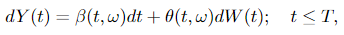
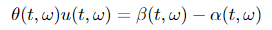
the place W(t) ∈ ℝᵐ, β ∈ ℝⁿ and θ ∈ ℝⁿˣᵐ. Suppose there exists processes u(t, ω) and α(t, ω) such that
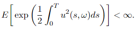
and assume that u(t, ω) satisfies Novikov’s situation
Let
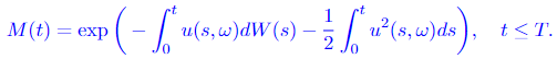
Measure P and Q are outlined in the identical approach as in Girsanov theorem I, which implies that E = Eₚ in Equation 3.3, and Equation 3.2 additionally applies. Then
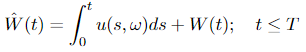
is a Wiener course of with regard to measure Q and the method Y(t) has one other illustration by way of W_hat(t)
Within the Girsanov theorem II, we are able to see that the drift of Y(t) modifications from β(t, ω) to α(t, ω). Additionally, as a aspect notice, processes u(t, ω) and α(t, ω) ought to fulfill sure situations, that are omitted right here to make the massive image clear.
The converse of the Girsanov theorem
In logic, the converse of a press release p → q is q → p. Within the Girasnov theorem, in easy phrases, p is the brand new measure, and q is the brand new course of. Then the converse is formulated (with regard to Girsanov I, as a result of it is simpler) as:
Let P be a Wiener measure of Wiener course of W(t) and let Q~P be an equal measure on (Ω, 𝓐). Then there exists a stochastic course of α(t, ω) ∈ ℝⁿ, 0 ≤ t ≤ T, tailored with regard to the historical past of W(t) (see Expression 3.0), such that

is a Wiener course of on the likelihood area (Ω, 𝓐, Q). And the corresponding Radon-Nikodym is given by Equation 3.1. For handy reference and the significance of this components, we paste it right here once more

Abstract
On this submit, we began with the continuity of likelihood distribution — discrete, completely steady, and singular steady. Then the Radon-Nikodym spinoff and concept are launched, which is key for the Girsanov theorem. Within the final part, the Girsanov theorem is launched. Two formulations of the Girsanov theorem are included, one is a change from the Wiener measure to a different measure, and one other one is switching between two totally different measures. Finally, we present the converse of the Girsanov theorem. A really fascinating and helpful software of the Girsanov theorem is to make an asset value modeled by the Black-Scholes components martingale. It isn’t included on this submit since it’s already prolonged sufficient. We’ll see it in an upcoming submit about monetary derivatives and the Black-Scholes components.:)
