
Let’s discover some strategies to adapt your parameters over time.

On this submit, I’ll talk about the concepts behind adaptive parameters strategies for machine studying and why and when to implement them as some sensible examples utilizing python.
Adaptive strategies (also referred to as parameter scheduling) confer with methods to replace some mannequin parameters at coaching time utilizing a schedule.
This alteration will rely upon the mannequin’s state at time t; for instance, you may set replace them relying on the loss worth, the variety of iterations/epochs, elapsed coaching time, and so forth.
For instance, generally, for neural networks, the selection of the educational charge has a number of penalties; if the educational charge is just too giant, it might overshoot the minimal; if it is too small, it might take it too lengthy to converge, or it’d get caught on a neighborhood minimal.

On this situation, we select to vary the educational charge as a perform of the epochs; this manner, you might set a big charge at the start of the coaching, and conforming to the epochs will increase; you may lower the worth till you attain a decrease threshold.
You may also see it as a approach of exploration vs. exploitation technique, so at the start, you enable extra exploration, and on the finish, you select exploitation.
There are a number of strategies you may select to regulate the shape and the pace from which the parameter goes from an preliminary worth to a ultimate threshold; on this article, I am going to name them “Adapters”, and I am going to deal with strategies that change the parameter worth as a perform of the variety of iterations (epochs in case of neural networks).
I am going to introduce some definitions and notation:
The preliminary worth represents the place to begin of the parameter, the end_value is the worth you’d get after many iterations, and the adaptive charge controls how briskly you go from the initial_value to the end_value.

Beneath this situation, you’d anticipate to have the next properties for every adapter:

On this article, I am going to clarify three sorts of adapters:
- Exponential
- Inverse
- Potential
The Exponential Adapter makes use of the next type to vary the preliminary worth:

From this components, alpha must be a optimistic worth to have the specified properties.
If we plot this adapter for various alpha values, we will see how the parameter worth decreases with completely different shapes, however all of them observe an exponential decay; this exhibits how the selection of alpha impacts the decay pace.
On this instance, the initial_value is 0.8, and the tip worth is 0.2. You possibly can see that bigger alpha values require fewer steps/iterations to converge to a price near 0.2.

If you choose the initial_value to be decrease than the end_value, you will be performing an exponential ascend, which will be useful in some instances; for instance, in genetic algorithms, you might begin with a low crossover chance on the first technology, and enhance it because the generations go ahead.
The next is how the above plot would look if the place to begin is 0.2 and goes till 0.8; you may see the symmetry towards the decay.

The Inverse Adapter makes use of the next type to vary the preliminary worth:

From this components, alpha must be a optimistic worth to have the specified properties. That is how the adapter appears:
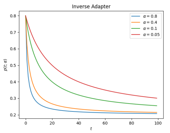
The Inverse Adapter makes use of the next type to vary the preliminary worth:

This components requires that alpha is within the vary (0, 1) to have the specified properties. That is how the adapter appears:

As we noticed, all of the adapters change the preliminary parameter at a unique charge (which is dependent upon alpha), so it is useful to see how they behave compared; that is the end result for a set alpha worth of 0.15.
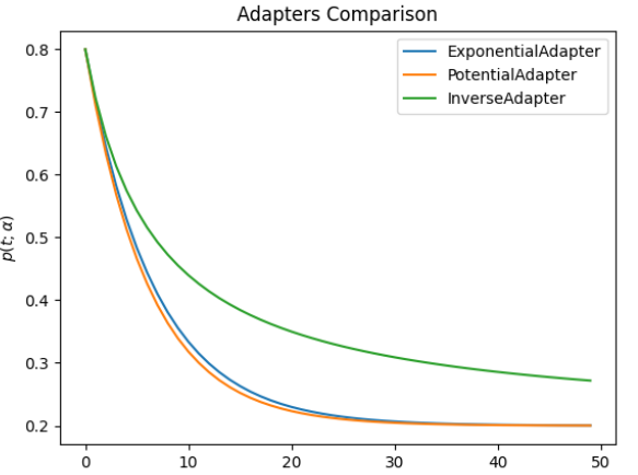
You possibly can see that the potential adapter is the one which decreases extra quickly, adopted very shut by the exponential; the inverse adapter might require an extended variety of iterations to converge.
That is the code used for this comparability in case you wish to play with the parameters to see its impact; first, be sure that to put in the package deal [2]:
pip set up sklearn-genetic-opt
On this part, we wish to use an algorithm for computerized hyperparameter tuning; such algorithms normally include choices to regulate de optimization course of; for instance, I will use a genetic algorithm to regulate the mutation and crossover chances with an exponential adapter; these are associated to the exploration vs. exploration technique of the algorithm.
You possibly can verify this different article I wrote to grasp extra about genetic algorithms for hyperparameter tuning.
First, allow us to import the package deal we require. I’ll use the digits dataset [1] and fine-tune a Random Forest mannequin.
Word: I am the writer of the package deal used within the instance; if you wish to know additional, contribute or make some solutions, you may verify the documentation and the GitHub repository on the finish of this text.
The para_grid parameter delimits the mannequin’s hyperparameters search area and defines the information varieties; we’ll use the cross-validation accuracy to guage the mannequin’s hyperparameters.
We outline the optimization algorithm and create the adaptive crossover and mutation chances. We’ll begin with a excessive mutation chance and a low crossover chance; because the generations enhance, the crossover and mutation chance will enhance and reduce, respectively.
We’ll additionally print and plot some statistics to grasp the outcomes.
On this specific instance, I acquired an accuracy rating of 0.941 (on check information) and located these parameters:
{‘min_weight_fraction_leaf’: 0.01079845233781555, ‘bootstrap’: True, ‘max_depth’: 10, ‘max_leaf_nodes’: 27, ‘n_estimators’: 108}
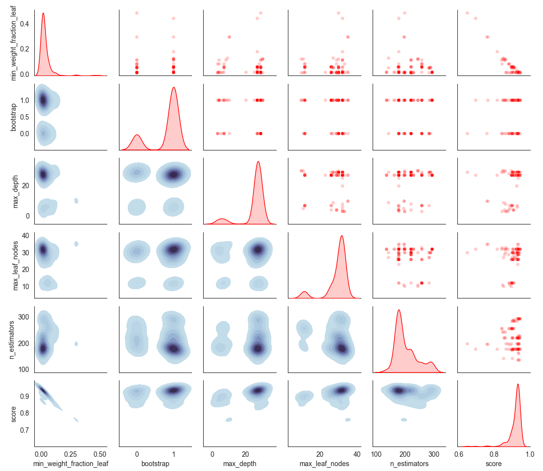
You possibly can verify the search area, which exhibits which hyperparameters had been explored by the algorithm.

For reference, that is how the sampled area appears with out adaptive studying; the algorithm explored fewer areas with a set low mutation chance (0.2) and a excessive crossover chance (0.8).
Adapting or scheduling parameters will be very helpful when coaching a machine studying algorithm; it’d assist you to converge the algorithm sooner or to discover complicated areas of area with a dynamic technique, even when the literature primarily makes use of them for deep studying, as we have proven, you can even use this for conventional machine studying, and adapt its concepts to increase it to some other set of issues that will swimsuit a altering parameter technique.
If you wish to know extra about sklearn-genetic-opt, you may verify the documentation right here:
[1] Digits Dataset beneath Artistic Commons Attribution 4.0 Worldwide (CC BY 4.0) license: https://archive-beta.ics.uci.edu/ml/datasets/optical+recognition+of+handwritten+digits
[2] sklearn-genetic-opt repo: https://github.com/rodrigo-arenas/Sklearn-genetic-opt
