An introduction to RNN, LSTM, and GRU and their implementation

If you wish to make predictions on sequential or time sequence information (e.g., textual content, audio, and many others.) conventional neural networks are a nasty alternative. However why?
In time sequence information, the present commentary relies on earlier observations, and thus observations should not unbiased from one another. Conventional neural networks, nevertheless, view every commentary as unbiased because the networks should not capable of retain previous or historic data. Bascially, they don’t have any reminiscence of what happend prior to now.
This led to the rise of Recurrent Neural Networks (RNNs), which introduce the idea of reminiscence to neural networks by together with the dependency between information factors. With this, RNNs could be educated to recollect ideas primarily based on context, i.e., be taught repeated patterns.
However how does an RNN obtain this reminiscence?
RNNs obtain a reminiscence by means of a suggestions loop within the cell. And that is the principle distinction between a RNN and a conventional neural community. The feed-back loop permits data to be handed inside a layer in distinction to feed-forward neural networks wherein data is simply handed between layers.
RNNs should then outline what data is related sufficient to be saved within the reminiscence. For this, various kinds of RNN developed:
- Conventional Recurrent Neural Community (RNN)
- Lengthy-Quick-term-Reminiscence Recurrent Neural Community (LSTM)
- Gated Recurrent Unit Recurrent Neural Community (GRU)
On this article, I offer you an introduction to RNN, LSTM, and GRU. I’ll present you their similarities and variations in addition to some benefits and disadvantges. Moreover the theoretical foundations I additionally present you how one can implement every strategy in Python utilizing tensorflow.
Via the suggestions loop the output of 1 RNN cell can also be used as an enter by the identical cell. Therefore, every cell has two inputs: the previous and the current. Utilizing data of the previous ends in a brief time period reminiscence.
For a greater understanding we unroll/unfold the suggestions loop of an RNN cell. The size of the unrolled cell is the same as the variety of time steps of the enter sequence.

We will see how previous observations are handed by means of the unfolded community as a hidden state. In every cell the enter of the present time step x (current worth), the hidden state h of the earlier time step (previous worth) and a bias are mixed after which restricted by an activation operate to find out the hidden state of the present time step.

Right here, the small, daring letters characterize vectors whereas the captial, daring letters characterize matrices.
The weights W of the RNN are up to date by means of a backpropagation in time (BPTT) algorithm.
RNNs can be utilized for one-to-one, one-to-many, many-to-one, and many-to-many predictions.
Benefits of RNNs
Attributable to their shortterm reminiscence RNNs can deal with sequential information and determine patterns within the historic information. Furthermore, RNNs are capable of deal with inputs of various size.
Disadvantages of RNNs
The RNN suffers from the vanishing gradient descent. On this, the gradients which might be used to replace the weights throughout backpropagation change into very small. Multiplying weights with a gradient that’s near zero prevents the community from studying new weights. This stopping of studying ends in the RNN forgetting what’s seen in longer sequences. The issue of vanishing gradient descent will increase the extra layers the community has.
Because the RNN solely retains latest data, the mannequin has issues to think about observations which lie far prior to now. The RNN, thus, tends to unfastened data over lengthy sequences because it solely shops the newest data. Therefore, the RNN has solely a short-term however not a long-term reminiscence.
Furthermore, because the RNN makes use of backpropagation in time to replace weights, the community additionally suffers from exploding gradients and, if ReLu activation capabilities are used, from useless ReLu items. The primary would possibly result in convergence points whereas the latter would possibly cease the training.
Implementation of RNNs in tensorflow
We will simply implement a RNN in Python utilizing tensorflow. For this, we use the Sequential mannequin which permits us to stack layers of RNN, i.e., the SimpleRNN layer class, and the Dense layer class.
from tensorflow.keras import Sequential
from tensorflow.keras.layers import SimpleRNN, Dense
from tensorflow.keras.optimizers import Adam
Importing the optimizer shouldn’t be essential so long as we need to use the default parameters. Nonetheless, if we need to customise any parameters of the optimizer we have to import the optimizer as properly.
To construct the community, we outline a Sequential mannequin after which use the add() technique so as to add the RNN layers. So as to add a RNN layer, we use the SimpleRNN class and move parameters, such because the variety of items, the dropout fee or the activation operate. For our first layer we will additionally move the form of our enter sequence.
If we stack RNN layers, we have to set the return_sequence parameter of the earlier layer to True. This ensures that the output of the layer has the proper format for the subsequent RNN layer.
To generate an output we use a Dense layer as our final layer, passing the variety of outputs.
# outline parameters
n_timesteps, n_features, n_outputs = X_train.form[1], X_train.form[2], y_train.form[1]# outline mannequin
rnn_model = Sequential()
rnn_model.add(SimpleRNN(130, dropout=0.2, return_sequences=True, input_shape=(n_timesteps, n_features)))
rnn_model.add(SimpleRNN(110, dropout=0.2, activation="tanh", return_sequences=True))
rnn_model.add(SimpleRNN(130, dropout=0.2, activation="tanh", return_sequences=True))
rnn_model.add(SimpleRNN(100, dropout=0.2, activation="sigmoid", return_sequences=True))
rnn_model.add(SimpleRNN(40, dropout=0.3, activation="tanh"))
rnn_model.add(Dense(n_outputs))
After we’ve outlined our RNN, we will compile the mannequin utilizing the compile() technique. Right here, we move the loss operate and the optimizer we need to use. tensorflow offers some built-in loss capabilities and optimizers.
rnn_model.compile(loss='mean_squared_error', optimizer=Adam(learning_rate=0.001))
Earlier than we practice the RNN, we will take a look on the mannequin and the variety of parameters, utilizing the abstract() technique. This may give us and overview in regards to the complexity of our mannequin.
We practice the mannequin utilizing the match() technique. Right here, we have to move the coaching information and completely different parameters to customise the coaching, together with the variety of epochs, the batch dimension, a validation cut up, and an early stopping.
stop_early = tf.keras.callbacks.EarlyStopping(monitor='val_loss', endurance=5)
rnn_model.match(X_train, y_train, epochs=30, batch_size=32, validation_split=0.2, callbacks=[stop_early])
To make predictions on our check information set or on any unseen information, we will use the predict() technique. The verbose parameter simply states if we need to get any data on the standing of the prediction course of. On this case, I didn’t need any print out of the standing.
y_pred = rnn_model.predict(X_test, verbose=0)
Hyperparameter tuning for RNNs in tensorflow
As we will see the implementation of an RNN is fairly easy. Discovering the proper hyperparameters, equivalent to variety of items per layer, dropout fee or activation operate, nevertheless, is way tougher.
However as a substitute of various the hyperparameter manually, we will use the keras-tuner library. The library has 4 tuners, RandomSearch, Hyperband, BayesianOptimization, and Sklearn, to determine the proper hyperparameter mixture from a given search area.
To run the tuner we first have to import tensorflow and the Keras Tuner.
import tensorflow as tf
import keras_tuner as kt
We then construct the mannequin for hypertuning, wherein we outline the hyperparameter search area. We will construct the hypermodel utilizing a operate, wherein we construct the mannequin in the identical manner as above described. The one distinction is that we add the search area for every hyperparameter we need to tune. Within the instance under, I need to tune the variety of items, the activation operate, and the dropout fee for every RNN layer.
def build_RNN_model(hp):# outline parameters
n_timesteps, n_features, n_outputs = X_train.form[1], X_train.form[2], y_train.form[1]
# outline mannequin
mannequin = Sequential()
mannequin.add(SimpleRNN(hp.Int('input_unit',min_value=50,max_value=150,step=20), return_sequences=True, dropout=hp.Float('in_dropout',min_value=0,max_value=.5,step=0.1), input_shape=(n_timesteps, n_features)))
mannequin.add(SimpleRNN(hp.Int('layer 1',min_value=50,max_value=150,step=20), activation=hp.Alternative("l1_activation", values=["tanh", "relu", "sigmoid"]), dropout=hp.Float('l1_dropout',min_value=0,max_value=.5,step=0.1), return_sequences=True))
mannequin.add(SimpleRNN(hp.Int('layer 2',min_value=50,max_value=150,step=20), activation=hp.Alternative("l2_activation", values=["tanh", "relu", "sigmoid"]), dropout=hp.Float('l2_dropout',min_value=0,max_value=.5,step=0.1), return_sequences=True))
mannequin.add(SimpleRNN(hp.Int('layer 3',min_value=20,max_value=150,step=20), activation=hp.Alternative("l3_activation", values=["tanh", "relu", "sigmoid"]), dropout=hp.Float('l3_dropout',min_value=0,max_value=.5,step=0.1), return_sequences=True))
mannequin.add(SimpleRNN(hp.Int('layer 4',min_value=20,max_value=150,step=20), activation=hp.Alternative("l4_activation", values=["tanh", "relu", "sigmoid"]), dropout=hp.Float('l4_dropout',min_value=0,max_value=.5,step=0.1)))
# output layer
mannequin.add(Dense(n_outputs))
mannequin.compile(loss='mean_squared_error', optimizer=Adam(learning_rate=1e-3))
return mannequin
To outline the search area for every variable we will use completely different strategies, equivalent to hp.Int, hp.Float, and hp.Alternative. The primary two are very related their use. We give them a reputation, a minimal worth, a most worth, and a step dimension. The title is used to determine the hyperparameter whereas the minimal and most worth outline our vary of values. The step parameters defines the values within the vary we use for the tuning. The hp.Alternative can be utilized to tune categorical hyperparameters such because the activation operate. Right here, we solely must move an inventory of the alternatives we need to check.
After we’ve constructed our hypermodel, we have to instantiate the tuner and carry out the hypertuning. Though we will select between completely different algorithms for the tuning, their instantiation may be very related. We typically have to specify the target to optimize and the utmost variety of epochs to coach. Right here, it’s endorsed to set the epochs to a quantity which is barely increased than our anticipated variety of epochs after which use early stopping.
For instance, if we need to use the Hyperband tuner and the validation loss as the target we will construct the tuner as
tuner = kt.Hyperband(build_RNN_model,
goal="val_loss",
max_epochs=100,
issue=3,
hyperband_iterations=5,
listing='kt_dir',
project_name='rnn',
overwrite=True)
Right here, I additionally handed the listing wherein the outcomes shall be saved and the way usually the tuner shall iterate over the complete Hyperband algorithm.
After we’ve instantiated the tuner, we will use the search() technique to carry out the hyperparameter tuning.
stop_early = tf.keras.callbacks.EarlyStopping(monitor='val_loss', endurance=5)
tuner.search(X_train, y_train, validation_split=0.2, callbacks=[stop_early])
To extract the optimum hyperparameters, we will then use the get_best_hyperparameters() technique and use the get() technique and the title of every hyperparameter we tuned.
best_hps=tuner.get_best_hyperparameters(num_trials=1)[0]
print(f"enter: {best_hps.get('input_unit')}")
print(f"enter dropout: {best_hps.get('in_dropout')}")
LSTMs are a particular sort of RNNs which deal with the principle drawback of easy RNNs, the issue of vanishing gradients, i.e., the lack of data that lies additional prior to now.

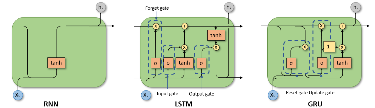
The important thing to LSTMs is the cell state, which is handed from the enter to the output of a cell. Thus, the cell state permits data to circulate alongside all the chain with solely minor linear actions by means of three gates. Therefore, the cell state represents the long-term reminiscence of the LSTM. The three gates are known as the neglect gate, enter gate, and ouput gate. These gates work as filters and management the circulate of knowledge and decide which data is saved or disregarded.
The neglect gate decides how a lot of the long-term reminiscence shall be saved. For this, a sigmoid operate is used which states the significance of the cell state. The output varies between 0 and 1 and states how a lot data is saved, i.e., 0, hold no data and 1, hold all data of the cell state. The output is set by combining the present enter x, the hidden state h of the earlier time step, and a bias b.

The enter gate decides which data shall be added to the cell state and thus the long-term reminiscence. Right here, a sigmoid layer decides which values are up to date.

The output gate decides which elements of the cell state construct the output. Therefore, the output gate is responsbile for the short-term reminiscence.

As could be seen, all three gates are represented by the identical operate. Solely the weights and biases differ. The cell state is up to date by means of the neglect gate and the enter gate.

The primary time period within the above equation determines how a lot of the long-term reminiscence is saved whereas the second phrases provides new data to the cell state.
The hidden state of the present time step is then decided by the output gate and a tanh operate which limits the cell state between -1 and 1.

Benefits of LSTMs
Some great benefits of the LSTM are just like RNNs with the principle profit being that they will seize patterns within the long-term and short-term of a sequence. Therefore, they’re probably the most used RNNs.
Disadvantages of LSTMs
Attributable to their extra complicated construction, LSTMs are computationally costlier, resulting in longer coaching instances.
Because the LSTM additionally makes use of the backpropagation in time algorithm to replace the weights, the LSTM suffers from the disadvantages of the backpropagation (e.g., useless ReLu components, exploding gradients).
Implementation of LSTMs in tensorflow
The implementation of LSTMs in tensorflow is similar to a easy RNN. The one distinction is that we import the LSTM class as a substitute of the SimpleRNN class.
from tensorflow.keras import Sequential
from tensorflow.keras.layers import LSTM, Dense
from tensorflow.keras.optimizers import Adam
We will the put collectively the LSTM community in the identical manner as the easy RNN.
# outline parameters
n_timesteps, n_features, n_outputs = X_train.form[1], X_train.form[2], y_train.form[1]# outline mannequin
lstm_model = Sequential()
lstm_model.add(LSTM(130, return_sequences=True, dropout=0.2, input_shape=(n_timesteps, n_features)))
lstm_model.add(LSTM(70, activation="relu", dropout=0.1, return_sequences=True))
lstm_model.add(LSTM(100, activation="tanh", dropout=0))
# output layer
lstm_model.add(Dense(n_outputs, activation="tanh"))
lstm_model.compile(loss='mean_squared_error', optimizer=Adam(learning_rate=0.001))
stop_early = tf.keras.callbacks.EarlyStopping(monitor='val_loss', endurance=5)
lstm_model.match(X_train, y_train, epochs=30, batch_size=32, validation_split=0.2, callbacks=[stop_early])
The hyperparameter tuning can also be the identical as for the easy RNN. Therefore, we solely have to make minor modifications to the code snippets I’ve proven above.
Much like LSTMs, the GRU solves the vanishing gradient drawback of easy RNNs. The distinction to LSTMs, nevertheless, is that GRUs use fewer gates and should not have a separate inner reminiscence, i.e., cell state. Therefore, the GRU solely depends on the hidden state as a reminiscence, resulting in an easier structure.

The reset gate is accountable for the short-term reminiscence because it decides how a lot previous data is saved and disregarded.

The values within the vector r are bounded between 0 and 1 by a sigmoid operate and depend upon the hidden state h of the earlier time step and the present enter x. Each are weighted utilizing the load matrices W. Moreover, a bias b is added.
The replace gate, in distinction, is accountable for the long-term reminiscence and is corresponding to the LSTM’s neglect gate.

As we will see the one distinction between the reset and replace gate are the weights W.
The hidden state of the present time step is set primarily based on a two step course of. First, a candidate hidden state is set. The candidate state is a mixture of the present enter and the hidden state of the earlier time step and an activation operate. On this instance, a tanh operate is used. The affect of the earlier hidden state on the candidate hidden state is managed by the reset gate

Within the second step, the candidate hidden state is mixed with the hidden state of the earlier time step to generate the present hidden state. How the earlier hidden state and the candidate hidden state are mixed is set by the replace gate.

If the replace gate provides a worth of 0 then the earlier hidden state is completly disregarded and the present hidden state is the same as the candidate hidden state. If the replace gate provides a worth of 1, it’s vice versa.
Benefits of GRUs
Because of the easier structure in comparison with LSTMs (i.e., two as a substitute of three gates and one state as a substitute of two), GRUs are computationally extra efficent and quicker to coach as they want much less reminiscence.
Furthermore, GRUs haven confirmed to be extra environment friendly for smaller sequences.
Disadvantages of GRUs
As GRUs should not have a separate hidden and cell state they won’t be capable to take into account observations as far into the previous because the LSTM.
SImilar to the RNN and LSTM, the GRU additionally would possibly undergo from the disadvantages of the backpropagation in time to replace the weights, i.e., useless ReLu components, exploding gradients.
Implementation of GRUs in tensorflow
As for the LSTM, the implementation of GRU is similar to easy RNN. We solely have to import the GRU class whereas the remainder stays the identical.
from tensorflow.keras import Sequential
from tensorflow.keras.layers import GRU, Dense
from tensorflow.keras.optimizers import Adam# outline parameters
n_timesteps, n_features, n_outputs = X_train.form[1], X_train.form[2], y_train.form[1]
# outline mannequin
gru_model = Sequential()
gru_model.add(GRU(90,return_sequences=True, dropout=0.2, input_shape=(n_timesteps, n_features)))
gru_model.add(GRU(150, activation="tanh", dropout=0.2, return_sequences=True))
gru_model.add(GRU(60, activation="relu", dropout=0.5))
gru_model.add(Dense(n_outputs))
gru_model.compile(loss='mean_squared_error', optimizer=Adam(learning_rate=0.001))
stop_early = tf.keras.callbacks.EarlyStopping(monitor='val_loss', endurance=5)
gru_model.match(X_train, y_train, epochs=30, batch_size=32, validation_split=0.2, callbacks=[stop_early])
The identical applies to the hyperparameter tuning.
