A recipe to empirically reply any query rapidly | by Quentin Gallea, PhD | Jul, 2022

From academia to company work, this recipe is for you

After years of doing scientific analysis, I ended up making a recipe to begin any analysis mission. This recipe, that I’m about to share with all of you, helps me day by day to have a really structured method, decreasing the danger of lacking one thing and maximizing effectivity.

You will notice that, as among the greatest chef, mastering the fundamentals is sufficient to give you one thing nice. That is additionally my method right here. You will notice no fancy instructions, lengthy strains of codes or sophisticated package deal to put in. This system allowed me to publish my three first scientific papers in among the most prestigious journals of their respecting fields: PNAS, Environmental Analysis Letters, or Administration Science (forthcoming).

Exploring knowledge could be painful, and boring, however additionally it is the place to begin to reply empirically any query (in academia or within the “actual” world). Therefore, it’s completely key to do that half cautiously.

Let me use a really concrete instance from my every day life as a researcher for instance my technique and see how we are able to shed gentle rapidly on a query, whereas hopefully having fun with the method.

Case research: A colleague of mine approached me in the course of the present warmth wave (June 2022), and she or he was questioning if such an occasion would assist to implement environmental insurance policies or not. Therefore, I’ve determined to make use of this query for instance my commonplace method to finding out the connection between two variables.

At every step I’ll clarify what I observe and the way it impacts my selections for the evaluation. That is the method I’ll collectively educate (with Boris Thurm and Edoardo Chiarotti) for the Grasp in Sustainable Administration and Know-how in the course of the spring semester (by Enterprise 4 Society at EPFL/UNIL/IMD). I’ll publish repeatedly comparable analyses with completely different kind of knowledge (you possibly can counsel what to discover subsequent within the feedback).

Disclaimer: This is step one after I need a first glimpse on the knowledge in a single hour or so. Clearly, each half could possibly be prolonged. Therefore, I put some notes for just a few issues that I’d discover in a second step.

The 5 steps for a great recipe:

1. Choosing the components for the recipe (how I choose the variables)
2. Choosing the right amount of every ingredient (how I choose my pattern)
3. Tasting and making ready the components (univariate evaluation)
4. Cooking the components collectively (bivariate evaluation)
5. Tasting the brand new recipe (conclusion).

1. Variables choice

On this part, I’ll simply conceptually take into consideration the connection between the weather and what are the important thing components I’ll want.

Central facet: Local weather change is a world, long-lasting, comparatively low tempo phenomenon. Therefore, the impact of warmth waves on climate-change legal guidelines is arguably causal (e.g. the habits of France in 2020 will not be anticipated to have an effect on the common temperature the identical yr or the yr after).

This primary half helps me to outline what are the variables I might want to begin my evaluation:

• final result: Environmental insurance policies,
• explanatory variable: Common yearly temperature,
• extra explanatory variable: Warmth-waves is perhaps aggravated if rainfall is low, therefore I can even add common yearly rainfall.

That is the minimal ingredient listing I would choose: an final result, an explanatory variable, and a 3rd variable to discover the potential heterogeneity of the impact (right here rainfall).

2. Pattern choice

On this part, I’ll search for the information availability to outline a transparent pattern. I’ll base my preliminary evaluation on the High quality of Authorities Environmental Indicators Dataset¹ which aggregates quite a few vital datasets with a whole lot of environmental variables.

Here’s a listing of the variables I chosen going via the codebook (hyperlink):
– cname: Nation title
– yr: Yr
– oecd_eps: Environmental Coverage Stringency Index² (from Botta and Kozluk (2014))
– cckp_temp: Annual common temperature in Celsius³ (from the Local weather Change Data Portal)
– cckp_rain: Annual common rainfall in mm³ (from the Local weather Change Data Portal)

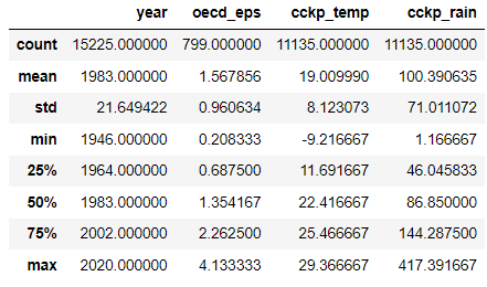
This primary desk reveals that the variable oecd_eps is on the market just for 799 observations.

Based mostly on the earlier tables, I’ll prohibit to the nations with knowledge for the result (oecd_eps) and to years from 1993 to 2012 to have a comparatively fixed pattern measurement. The clear “bottle neck” from the desk above is the result variable oecd_eps. Clearly, as a result of it’s targeted solely on OECD nations.

From the ‘depend’ line, we are able to see that the pattern has no lacking values.

Virtually completely balanced panel dataset (similar variety of observations for every unit/nation) with Brazil and Slovenia with fewer years.

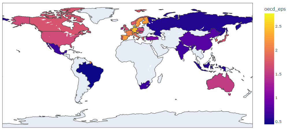
The map above exhibits that OECD nations (contained within the pattern) cowl each continent (besides Antarctica). Africa is represented solely by South Africa, whereas South America has solely Brazil. Observe that the small yellow half above Brazil is an abroad division of France: French Guiana. Therefore, it’s vital to remember that Europe, represents a big a part of the dataset, which finally will drive the outcomes.

On this part, I’ll use descriptive statistics to:

1. Put together the information: By finding out the distribution of the variables, I’ll see if I ought to remodel the information (e.g. log-transform, outline a categorical variable, take care of outliers, and so forth.)
2. Select the proper statistical instruments: After this step, I’ll know the character of every variable (steady, categorical, binary, and so forth) which permits me to decide on the proper statistical instruments (correlation, bar/line graphs, scatter plot, and so forth).
3. Get an concept of the underlying variation: I additionally discover it vital to take a look at how the variable varies over time (line graph) and house (map). It helps me to get a greater understanding of the information and doubtlessly spot some anomalies or attention-grabbing shocks to use for a pure experiment.

3.1 Final result variable: Environmental Coverage Stringency Index

• The Stringency index is a steady variable taking values from 0.3 and 4.1 inside the pattern chosen.
• The imply is 1.6 with a median barely decrease (1.5).

Observations:

1. Histogram and desk: The info are barely uneven on the proper (skewness 0.48) with a density of very low values. The skewness is a measure of asymmetry. Unfavorable values imply that there’s an asymmetry on the left, a null worth signifies that the distribution is completely symmetric whereas optimistic values suggest an asymmetry on the proper.
2. Map: Evidently the stringency of the environmental insurance policies is extremely correlated with GDP: Europe, North America, or Australia have excessive values whereas African, Asian or South American nations have lowers values. Therefore, it will be vital to take this into consideration for the multivariate evaluation (e.g. embody as management variable in a regression mannequin).
3. Line graph: General there’s a optimistic development. There may be additionally an attention-grabbing drop in 2007. I’d attempt to discover this later to search out out whether it is pushed by a subset of nations.

Now that I picked the portions and ready the components, I’ll put them collectively. My final result and explanatory variables are steady variables. Therefore, I’ll begin with a easy scatter plot because it stays very near the information, permits me to see every knowledge level, and ample given the pattern measurement (with hundreds of thousands of datapoints I’d favor a hexplot for instance).

That can assist you observe the steps, I put my observations after every graph.

Observations: Evidently the dots are unfold in small teams vertically. I assume that the common annual temperature have larger between-country variation than within-country. Therefore, it makes extra sense for the evaluation to take a look at how within-country variations in temperature are related to the result. To verify this concept I’ll merely plot the identical graph whereas coloring the dots by nations.

Remark: Certainly the temperature is comparatively secure over time, whereas there’s vital variation for the stringency index within-country.

Therefore, allow us to compute the distinction from the imply for the temperature variable for every nation relatively than utilizing the extent (within-country variation).

Remark: The connection is clearer and as anticipated it’s optimistic.

Subsequent? Heterogeneity: Now let’s look if there’s some heterogeneity with respect to rainfall.

Remark: Visually the connection is unclear. Nonetheless, the nations with the very best rain appear to have a low-temperature variation and low environmental coverage stringency index (doubtlessly Indonesia).

Let’s do a pattern break up to discover the connection between temperature and environmental coverage stringency index for nations with rainfall above versus under median (heterogeneity train).

Remark: The correlation between environmental coverage and temperature (deviation from the imply) is optimistic. The correlation is sort of zero for the pattern with rain above median (0.036) whereas it’s comparatively giant for the pattern above median (0.19). From the final graph, we are able to see that the slope of the linear match is steeper for the pattern with low rain however the intercept is decrease. It will be heroic to conclude something from these easy preliminary graphs. Nonetheless, it suggests some potential attention-grabbing heterogeneity. That is so far as I’ll go along with the descriptive statistics (already greater than a bivariate evaluation by the way in which).

What have we discovered from this exploration? First, it allowed me to point out you my recipe. Second, we discovered finally new issues concerning the relationship between temperature and environmental insurance policies:

1. There’s a optimistic affiliation between (within-country) temperature variation and environmental coverage stringency index (for OECD nations from 1993 to 2012).
2. The connection is strongly strengthened for observations experiencing low rain throughout the identical yr.
3. From this easy heterogeneity train, it stays unclear if this affiliation is stronger for nations the place there’s little rain on common (e.g.: Australia, Spain, or South Africa) or for any nation throughout drier years (e.g.: France in 2003).

Subsequent: I’d now refine this train and particularly look into three issues: 1. What occurred in 2007 with the drop within the stringency index (one nation, all nations, and perceive why), 2. Discover additionally which areas are driving the aggregated drop in temperature in 1998 and 2010 (it may result in an attention-grabbing occasion research). 3. Use an occasion research to examine if the impact takes place solely the identical yr, or with lags and so forth. Then, relying on the findings, I’d match a multivariate mannequin to quantify the impact and management for cofounders.

[1] Povitkina, Marina, Natalia Alvarado Pachon, and Cem Mert Dalli. “The High quality of Authorities Environmental Indicators Dataset, model Sep21.” College of Gothenburg: The High quality of Authorities Institute, https://www. gu.se/en/quality-government (2021).

[2] Botta, Enrico, and Tomasz Koźluk. “Measuring environmental coverage stringency in OECD nations: A composite index method.” (2014).

[3] The World Financial institution Group. 2021. Local weather Change Data Portal. url: https://climateknowledgeportal.worldbank.org

[3] Harris, Ian, et al. “Model 4 of the CRU TS month-to-month high-resolution gridded multivariate local weather dataset.” Scientific knowledge 7.1 (2020): 1–18.