A number of Linear Regression With scikit-learn

On this article, let’s study a number of linear regression utilizing scikit-learn within the Python programming language.

Regression is a statistical technique for figuring out the connection between options and an end result variable or outcome. Machine studying, it’s utilized as a technique for predictive modeling, during which an algorithm is employed to forecast steady outcomes. A number of linear regression, typically referred to as a number of regression, is a statistical technique that predicts the results of a response variable by combining quite a few explanatory variables. A number of regression is a variant of linear regression (extraordinary least squares)  during which only one explanatory variable is used.

Mathematical Imputation:

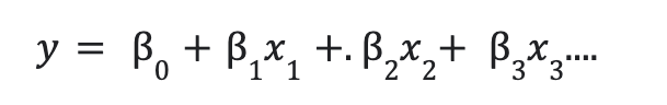
To enhance prediction, extra unbiased elements are mixed. The next is the linear relationship between the dependent and unbiased variables:

 

right here, y is the dependent variable.

• x1, x2,x3,… are unbiased variables.
• b0 =intercept of the road.
• b1, b2, … are coefficients.

for a easy linear regression line is of the shape :

y = mx+c

for instance if we take a easy instance, :

characteristic 1: TV

characteristic 2: radio

characteristic 3:  Newspaper

output variable: gross sales

Unbiased variables are the options feature1 , characteristic 2 and have 3. Dependent variable is gross sales. The equation for this downside might be:

y = b0+b1x1+b2x2+b3x3

x1, x2 and x3 are the characteristic variables. 

On this instance, we use scikit-learn to carry out linear regression. As we have now a number of characteristic variables and a single end result variable, it’s a A number of linear regression. Let’s see how to do that step-wise.

Stepwise Implementation

Step 1: Import the required packages

The required packages akin to pandas, NumPy, sklearn, and many others… are imported.

Step 2: Import the CSV file:

The CSV file is imported utilizing pd.read_csv() technique. To entry the CSV file click on right here. The ‘No ‘ column is dropped as an index is already current. df.head() technique is used to retrieve the primary 5 rows of the dataframe. df.columns attribute returns the title of the columns. The column names beginning with ‘X’ are the unbiased options in our dataset. The column ‘Y home worth of unit space’ is the dependent variable column. Because the variety of unbiased or exploratory variables is a couple of, it’s a Multilinear regression.

To view and obtain the CSV file click on right here.

Output:

   X1 transaction date  X2 home age  …  X6 longitude  Y home worth of unit space

0             2012.917          32.0  …     121.54024                        37.9

1             2012.917          19.5  …     121.53951                        42.2

2             2013.583          13.3  …     121.54391                        47.3

3             2013.500          13.3  …     121.54391                        54.8

4             2012.833           5.0  …     121.54245                        43.1

[5 rows x 7 columns]

Index([‘X1 transaction date’, ‘X2 house age’,

      ‘X3 distance to the nearest MRT station’,

      ‘X4 number of convenience stores’, ‘X5 latitude’, ‘X6 longitude’,

      ‘Y house price of unit area’],

     dtype=’object’)

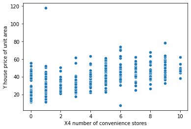
Step 3: Create a scatterplot to visualise the information:

A scatterplot is created to visualise the relation between the ‘X4 variety of comfort shops’ unbiased variable and the ‘Y home worth of unit space’ dependent characteristic.

Output:

 

Step 4: Create characteristic variables: 

To mannequin the information we have to create characteristic variables, X variable incorporates unbiased variables and y variable incorporates a dependent variable. X and Y characteristic variables are printed to see the information.

Output:

    X1 transaction date  X2 home age  …  X5 latitude  X6 longitude

0               2012.917          32.0  …     24.98298     121.54024

1               2012.917          19.5  …     24.98034     121.53951

2               2013.583          13.3  …     24.98746     121.54391

3               2013.500          13.3  …     24.98746     121.54391

4               2012.833           5.0  …     24.97937     121.54245

..                   …           …  …          …           …

409             2013.000          13.7  …     24.94155     121.50381

410             2012.667           5.6  …     24.97433     121.54310

411             2013.250          18.8  …     24.97923     121.53986

412             2013.000           8.1  …     24.96674     121.54067

413             2013.500           6.5  …     24.97433     121.54310

[414 rows x 6 columns]

0      37.9

1      42.2

2      47.3

3      54.8

4      43.1

      … 

409    15.4

410    50.0

411    40.6

412    52.5

413    63.9

Title: Y home worth of unit space, Size: 414, dtype: float64

Step 5: Cut up information into practice and take a look at units:

Right here, train_test_split() technique is used to create practice and take a look at units, the characteristic variables are handed within the technique. take a look at measurement is given as 0.3, which suggests 30% of the information goes into take a look at units, and practice set information incorporates 70% information. the random state is given for information reproducibility.

Step 6: Create a linear regression mannequin

A easy linear regression mannequin is created. LinearRegression() class is used to create a easy regression mannequin, the category is imported from sklearn.linear_model bundle.

Step 7: Match the mannequin with coaching information.

After creating the mannequin, it suits with the coaching information. The mannequin features information in regards to the statistics of the coaching mannequin. match() technique is used to suit the information.

Step 8: Make predictions on the take a look at information set.

On this mannequin.predict() technique is used to make predictions on the X_test information, as take a look at information is unseen information and the mannequin has no information in regards to the statistics of the take a look at set. 

Step 9: Consider the mannequin with metrics.

The multi-linear regression mannequin is evaluated with mean_squared_error and mean_absolute_error metric. when put next with the imply of the goal variable, we’ll perceive how effectively our mannequin is predicting. mean_squared_error is the imply of the sum of residuals. mean_absolute_error is the imply of absolutely the errors of the mannequin. The much less the error, the higher the mannequin efficiency is.

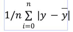
imply absolute error = it’s the imply of the sum of absolutely the values of residuals.

 

imply sq. error =  it’s the imply of the sum of the squares of residuals.

 

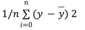
• y= precise worth
• y hat = predictions

Output:

mean_squared_error :  46.21179783493418
mean_absolute_error :  5.392293684756571

For information assortment, there must be a big discrepancy between the numbers. If you wish to ignore outliers in your information, MAE is a preferable various, however if you wish to account for them in your loss operate, MSE/RMSE is the way in which to go. MSE is all the time greater than MAE generally, MSE equals MAE solely when the magnitudes of the errors are the identical.

Code:

Right here, is the complete code collectively, combining the above steps.

Output:

   X1 transaction date  X2 home age  …  X6 longitude  Y home worth of unit space

0             2012.917          32.0  …     121.54024                        37.9

1             2012.917          19.5  …     121.53951                        42.2

2             2013.583          13.3  …     121.54391                        47.3

3             2013.500          13.3  …     121.54391                        54.8

4             2012.833           5.0  …     121.54245                        43.1

[5 rows x 7 columns]

Index([‘X1 transaction date’, ‘X2 house age’,

      ‘X3 distance to the nearest MRT station’,

      ‘X4 number of convenience stores’, ‘X5 latitude’, ‘X6 longitude’,

      ‘Y house price of unit area’],

     dtype=’object’)

    X1 transaction date  X2 home age  …  X5 latitude  X6 longitude

0               2012.917          32.0  …     24.98298     121.54024

1               2012.917          19.5  …     24.98034     121.53951

2               2013.583          13.3  …     24.98746     121.54391

3               2013.500          13.3  …     24.98746     121.54391

4               2012.833           5.0  …     24.97937     121.54245

..                   …           …  …          …           …

409             2013.000          13.7  …     24.94155     121.50381

410             2012.667           5.6  …     24.97433     121.54310

411             2013.250          18.8  …     24.97923     121.53986

412             2013.000           8.1  …     24.96674     121.54067

413             2013.500           6.5  …     24.97433     121.54310

[414 rows x 6 columns]

0      37.9

1      42.2

2      47.3

3      54.8

4      43.1

      … 

409    15.4

410    50.0

411    40.6

412    52.5

413    63.9

Title: Y home worth of unit space, Size: 414, dtype: float64

mean_squared_error :  46.21179783493418

mean_absolute_error :  5.392293684756571