A stepwise information for effectively explaining your fashions utilizing SHAP.
Introduction to MLlib
Apache Spark’s Machine Studying Library (MLlib) is designed primarily for scalability and pace by leveraging the Spark runtime for frequent distributed use circumstances in supervised studying like classification and regression, unsupervised studying like clustering and collaborative filtering and in different circumstances like dimensionality discount. On this article, I cowl how we will use SHAP to clarify a Gradient Boosted Timber (GBT) mannequin that has match our knowledge at scale.
What are Gradient Boosted Timber?
Earlier than we perceive what Gradient Boosted Timber are, we have to perceive boosting. Boosting is an ensemble method that sequentially combines quite a lot of weak learners to realize an total robust learner. In case of Gradient Boosted Timber, every weak learner is a call tree that sequentially minimizes the errors (MSE in case of regression and log loss in case of classification) generated by the earlier choice tree in that sequence. To examine GBTs in additional element, please discuss with this weblog publish.
Understanding our imports
from pyspark.sql import SparkSession
from pyspark import SparkContext, SparkConf
from pyspark.ml.classification import GBTClassificationModel
import pyspark.sql.capabilities as F
from pyspark.sql.varieties import *
The primary two imports are for initializing a Spark session. It will likely be used for changing our pandas dataframe to a spark one. The third import is used to load our GBT mannequin into reminiscence which might be handed to our SHAP explainer to generate explanations. The penultimate and final import is for performing SQL capabilities and utilizing SQL varieties. These might be utilized in our Consumer-Outlined Operate (UDF) which I shall describe later.
Changing our MLlib GBT characteristic vector to a Pandas dataframe
The SHAP Explainer takes a dataframe as enter. Nevertheless, coaching an MLlib GBT mannequin requires knowledge preprocessing. Extra particularly, the specific variables in our knowledge must be transformed into numeric variables utilizing both Class Indexing or One-Scorching Encoding. To be taught extra about methods to prepare a GBT mannequin, discuss with this article). The ensuing “options” column is a SparseVector (to learn extra on it, verify the “Preprocess Information” part in this instance). It seems to be like one thing beneath:
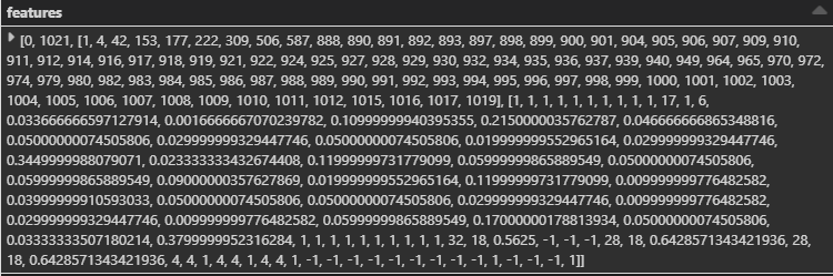
The “options” column proven above is for a single coaching occasion. We have to rework this SparseVector for all our coaching situations. One technique to do it’s to iteratively course of every row and append to our pandas dataframe that we are going to feed to our SHAP explainer (ouch!). There’s a a lot quicker means, which leverages the truth that we now have all of our knowledge loaded in reminiscence (if not, we will load it in batches and carry out the preprocessing for every in-memory batch). In Shikhar Dua’s phrases:
1. Create an inventory of dictionaries during which every dictionary corresponds to an enter knowledge row.
2. Create a knowledge body from this record.
So, primarily based on the above technique, we get one thing like this:
rows_list = []
for row in spark_df.rdd.acquire():
dict1 = {}
dict1.replace({ok:v for ok,v in zip(spark_df.cols,row.options)})
rows_list.append(dict1)
pandas_df = pd.DataFrame(rows_list)
If rdd.acquire() seems to be scary, it’s truly fairly easy to clarify. Resilient Distributed Datasets (RDD) are elementary Spark knowledge constructions which might be an immutable distribution of objects. Every dataset in an RDD is additional subdivided into logical partitions that may be computed in numerous employee nodes of our Spark cluster. So, all PySpark RDD acquire() does is retrieve knowledge from all of the employee nodes to the motive force node. As you may guess, it is a reminiscence bottleneck, and if we’re dealing with knowledge bigger than our driver node’s reminiscence capability, we have to improve the variety of our RDD partitions and filter them by partition index. Learn how to do this right here.
Don’t take my phrase on the execution efficiency. Try the stats.
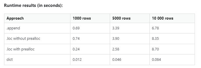
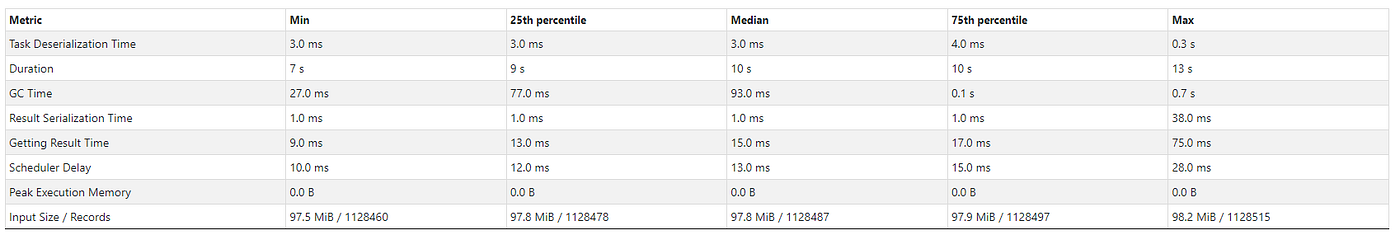
Listed here are the metrics from certainly one of my Databricks pocket book scheduled job runs:
Enter dimension: 11.9 GiB (~12.78GB), Complete time Throughout All Duties: 20 min, Variety of information: 165.16K
Working with the SHAP Library
We at the moment are able to cross our preprocessed dataset to the SHAP TreeExplainer. Do not forget that SHAP is a neighborhood characteristic attribution technique that explains particular person predictions as an algebraic sum of the shapley values of the options of our mannequin.
We use a TreeExplainer for the next causes:
- Appropriate: TreeExplainer is a category that computes SHAP values for tree-based fashions (Random Forest, XGBoost, LightGBM, GBT, and so forth).
- Precise: As an alternative of simulating lacking options by random sampling, it makes use of the tree construction by merely ignoring choice paths that depend on the lacking options. The TreeExplainer output is subsequently deterministic and doesn’t fluctuate primarily based on the background dataset.
- Environment friendly: As an alternative of iterating over every doable characteristic mixture (or a subset thereof), all mixtures are pushed by way of the tree concurrently, utilizing a extra complicated algorithm to maintain monitor of every mixture’s outcome — lowering complexity from O(TL2ᵐ) for all doable coalitions to the polynomial O(TLD²) (the place m is the variety of options, T is variety of bushes, L is most variety of leaves and D is most tree depth).
The check_additivity = False flag runs a validation verify to confirm if the sum of SHAP values equals to the output of the mannequin. Nevertheless, this flag requires predictions to be run that aren’t supported by Spark, so it must be set to False as it’s ignored anyway. As soon as we get the SHAP values, we convert it right into a pandas dataframe from a Numpy array, in order that it’s simply interpretable.
One factor to notice is that the dataset order is preserved after we convert a Spark dataframe to pandas, however the reverse is just not true.
The factors above lead us to the code snippet beneath:
gbt = GBTClassificationModel.load('your-model-path')
explainer = shap.TreeExplainer(gbt)
shap_values = explainer(pandas_df, check_additivity = False)
shap_pandas_df = pd.DataFrame(shap_values.values, cols = pandas_df.columns)
An Introduction to Pyspark UDFs and when to make use of them

Consumer-Outlined Features are complicated customized capabilities that function on a specific row of our dataset. These capabilities are typically used when the native Spark capabilities aren’t deemed enough to resolve the issue. Spark capabilities are inherently quicker than UDFs as a result of it’s natively a JVM construction whose strategies are carried out by native calls to Java APIs. Nevertheless, PySpark UDFs are Python implementations that requires knowledge motion between the Python interpreter and the JVM (discuss with Arrow 4 within the image above). This inevitably introduces some processing delay.
If no processing delays may be tolerated, the very best factor to do is create a Python wrapper to name the Scala UDF from PySpark itself. An excellent instance is proven in this weblog. Nevertheless, utilizing a PySpark UDF was enough for my use case, since it’s simple to grasp and code.
The code beneath explains the Python operate to be executed on every employee/executor node. We simply choose up the very best SHAP values (absolute values as we wish to discover probably the most impactful unfavourable options as effectively) and append it to the respective pos_features and neg_features record and in flip append each these lists to a options record that’s returned to the caller.
def shap_udf(row):
dict = {}
pos_features = []
neg_features = []
for characteristic in row.columns:
dict[feature] = row[feature]     dict_importance = {key: worth for key, worth in
sorted(dict.gadgets(), key=lambda merchandise: __builtin__.abs(merchandise[1]),
reverse = True)}     for ok,v in dict_importance.gadgets():
if __builtin__.abs(v) >= <your-threshold-shap-value>:
if v > 0:
pos_features.append((ok,v))
else:
neg_features.append((ok,v))
options = []
options.append(pos_features[:5])
options.append(neg_features[:5])    return options
We then register our PySpark UDF with our Python operate identify (in my case, it’s shap_udf) and specify the return kind (necessary in Python and Java) of the operate within the parameters to F.udf(). There are two lists within the outer ArrayType(), one for optimistic options and the opposite for unfavourable ones. Since every particular person record includes of at most 5 (feature-name, shap-value) StructType() pairs, it represents the interior ArrayType(). Under is the code:
udf_obj = F.udf(shap_udf, ArrayType(ArrayType(StructType([ StructField(‘Feature’, StringType()),
StructField(‘Shap_Value’, FloatType()),
]))))
Now, we simply create a brand new Spark dataframe with a column known as ‘Shap_Importance’ that invokes our UDF for every row of the spark_shapdf dataframe. To separate the optimistic and unfavourable options, we create two columns in a brand new Spark dataframe known as final_sparkdf. Our last code-snippet seems to be like beneath:
new_sparkdf = spark_df.withColumn(‘Shap_Importance’, udf_obj(F.struct([spark_shapdf[x] for x in spark_shapdf.columns])))final_sparkdf = new_sparkdf.withColumn(‘Positive_Shap’, final_sparkdf.Shap_Importance[0]).withColumn(‘Negative_Shap’, new_sparkdf.Shap_Importance[1])
And eventually, we now have extracted all of the essential options of our GBT mannequin per testing occasion with out the usage of any express for loops! The consolidated code may be discovered within the beneath GitHub gist.
P.S. That is my first try at writing an article and if there are any factual or statistical inconsistencies, please attain out to me and I shall be more than pleased to be taught along with you! 
