Half 3: Histograms & Density Plots
A Monte Carlo Simulation (MCS) is a sampling experiment whose purpose is to estimate the distribution of a amount of curiosity that depends upon a number of stochastic enter variables.
The event of an MCS entails three fundamental steps:
1. Arrange a predictive mannequin clearly figuring out the dependent variable (end result, unknown amount of curiosity, perform to be evaluated) and the impartial variables (random enter variables).
2. Determine the likelihood distributions of the enter variables. The usual process entails analyzing empirical or historic knowledge and becoming the information to a selected distribution. When such knowledge just isn’t out there, choose an applicable likelihood distribution and select properly its parameters.
3. Repeat the simulation a major variety of occasions acquiring random values of the output or dependent variable. Use statistical strategies to calculate some descriptive statistical measures and draw charts corresponding to histograms or density plots of the end result variable.
As indicated in a earlier article, we are able to use a Monte Carlo simulation to quantitatively account for danger in enterprise or operations administration duties.
A sensible utility of a Monte Carlo Simulation consists of manufacturing operations the place time between machine failures and their corresponding restore occasions are random variables.
Assume an enormous manufacturing unit the place a processing unit runs 24 hours per day, 335 days per 12 months (30 days for personnel holidays and yearly upkeep). Administration desires to purchase one other processing unit to elaborate on one other last product. They know that such processing models incur in random mechanical failures that require a extremely expert restore crew. So, each breakdown represents an necessary value.
The administration determined to conduct a Monte Carlo Simulation to numerically assess the chance related to the brand new challenge.
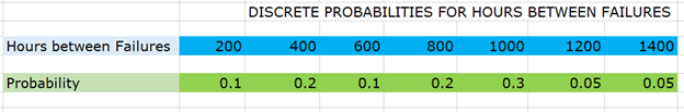
Historic knowledge of the current processing unit reveals that the time between machine failures has the next empirical distribution:
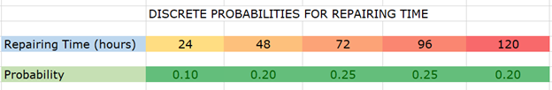
The time required to restore such a processing unit has the next empirical distribution:
The next Python code permits us to develop an MCS to numerical assess the chance concerned within the new funding:
First, we imported a number of Python libraries:
NumPy: a library for the Python programming language that gives help for creating giant multidimensional vectors and matrices, together with a big assortment of high-level mathematical capabilities to function on them.
SciPy: a free and open supply library for Python. Based mostly on NumPy, accommodates modules for statistics, linear algebra, optimization, interpolation, sign processing, and different typical strategies for science and engineering.
Matplotlib and Seaborn are conventional Python libraries for charting.
PrettyTable is a Python library for simply displaying tabular knowledge in a visually interesting ASCII desk format.
@creator: darwt
"""# Import Modules
import numpy  as npfrom scipy import stats
from scipy.stats import semimport matplotlib.pyplot as plt
import seaborn as sns
from prettytable import PrettyTableyour_path = 'your path'
Now we point out the working hours per 12 months, the hourly value incurred by the restore crew, the empirical distribution for hours of operation between failures, and the empirical distribution wanted for repairing.
# initialization moduleOperating_hours_year = 335 * 24
Cost_LostTime_hour = 55.50
# .........................................
# historic knowledge of hours of operation between failures (HbF)
Hours_between_Failures = [200, 400, 600, 800, 1000, 1200, 1400]# discrete chances for hours of operation between failures
probabilities_HBF = [0.1, 0.2, 0.1, 0.2, 0.3, 0.05, 0.05]# historic knowledge of hours wanted to restore (TTR)
Time_to_Repair = [24, 48, 72, 96, 120]probabilities_TTR =[0.10, 0.20, 0.25, 0.25, 0.20]
We set an enormous variety of replications, so our pattern imply will probably be very near the anticipated worth. We additionally outlined the extent of confidence for our Confidence Interval (CI).
Number_of_Replications = 2000confidence = 0.95                      ## chosen by the analyst# Lists to be stuffed throughout calculations
list_of_HBF,    list_of_TTR = [], []
list_Lost_Time, list_cost_TTR = [], []
list_Hours_Prod = []
The logic behind the MCS is described within the following strains of code. We’ve two loops: the outer loop (for run in vary(Number_of_Replication) associated to the variety of runs or replications; the inside loop (whereas acum_time <= Operating_hours_year ) associated to the yearly manufacturing and breakdowns. We used twice np.random.alternative to generate a random pattern of dimension one from each empirical distributions in accordance with their corresponding chances.
for run in vary(Number_of_Replications):
acum_time, acum_hbf, acum_ttr = 0, 0, 0
whereas acum_time <= Operating_hours_year:
HBF = np.random.alternative(Hours_between_Failures,
1, p=listing(probabilities_HBF))
TTR = np.random.alternative(Time_to_Repair,
1, p=listing(probabilities_TTR))
acum_time += (HBF + TTR)
acum_hbf += HBF
acum_ttr +=TTRTotal_HBF = spherical(float(acum_hbf),4)
Total_TTR = spherical(float(acum_ttr),4)
Perc_lost_Time = spherical(float(Total_TTR/Total_HBF * 100),2)
Hours_Prod = Operating_hours_year - Total_TTR
Cost_TTR = Total_TTR * Cost_LostTime_hour
list_of_HBF.append(Total_HBF)
list_of_TTR.append(Total_TTR)
list_Lost_Time.append(Perc_lost_Time)
list_cost_TTR.append(Cost_TTR)
list_Hours_Prod.append(Hours_Prod)
We used NumPy and SciPy to calculate key descriptive statistical measures, notably a Percentile Desk for our principal end result Cost_TTR = Total_TTR * Cost_LostTime_hour. This output variable represents the fee related to machine failures and the corresponding restore occasions. media represents the anticipated worth of such value.
media = spherical(np.imply(list_cost_TTR),2)
median = spherical(np.median(list_cost_TTR),2)
var = spherical(np.var(list_cost_TTR), 2)
stand = spherical(np.std(list_cost_TTR),2)std_error = spherical(sem(list_cost_TTR),2)skew = spherical(stats.skew(list_cost_TTR),2)
kurt = spherical(stats.kurtosis(list_cost_TTR),2)minimal = spherical(np.min(list_cost_TTR),2)
most = spherical(np.max(list_cost_TTR),2)dof = Number_of_Replications - 1
t_crit = np.abs(stats.t.ppf((1-confidence)/2,dof))half_width = spherical(stand *t_crit/np.sqrt(Number_of_Replications),2)
inf = media - half_width
sup = media + half_widthinf = spherical(float(inf),2)
sup = spherical(float(sup),2)
We used PrettyTable for the statistic report and the percentile report:
t = PrettyTable(['Statistic', 'Value'])
t.add_row(['Trials', Number_of_Replications])
t.add_row(['Mean', media])
t.add_row(['Median', median])
t.add_row(['Variance', var])
t.add_row(['Stand Dev', stand])
t.add_row(['Skewness', skew])
t.add_row(['Kurtosis', kurt])
t.add_row(['Half Width', half_width])
t.add_row(['CI inf', inf])
t.add_row(['CI sup', sup])
t.add_row(['Minimum', minimum])
t.add_row(['Maximum', maximum])
print(t)percents = np.percentile(list_cost_TTR, [10, 20, 30, 40, 50, 60, 70, 80, 90, 100])p = PrettyTable(['Percentile (%)', 'Lost Time Cost'])
p.add_row(['  10  ', percents[0]])
p.add_row(['  20  ', percents[1]])
p.add_row(['  30  ', percents[2]])
p.add_row(['  40  ', percents[3]])
p.add_row(['  50  ', percents[4]])
p.add_row(['  60  ', percents[5]])
p.add_row(['  70  ', percents[6]])
p.add_row(['  80  ', percents[7]])
p.add_row(['  90  ', percents[8]])
p.add_row([' 100  ', percents[9]])
print(p)
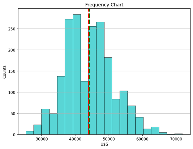
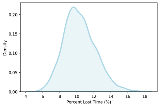
Lastly, we used Matplotlib and Seaborn for charting: a histogram that reveals the underlying frequency distribution of the anticipated misplaced time value per 12 months and a density plot that reveals the likelihood density perform of the p.c misplaced time resulting from breakdowns and repairs.
# Misplaced Time Value Histogramn_bins = 20fig, ax = plt.subplots(figsize=(8, 6))
ax.hist(list_cost_TTR, histtype ='bar', bins=20, coloration = 'c',
edgecolor='ok', alpha=0.65, density = False) # density=False present countsax.axvline(media, coloration='g', linestyle='dashed', linewidth=3)
ax.axvline(median, coloration='r', linestyle='dashed', linewidth=3)ax.set_title('Frequency Chart')
plt.savefig(your_path +'Anticipated Misplaced Time Value per 12 months',
ax.set_ylabel('Counts')
ax.set_xlabel('U$S')
ax.grid(axis = 'y')
bbox_inches='tight', dpi=150)
plt.present()# % Misplaced Time Value Density Plotsns.distplot(list_Lost_Time, hist=False, kde=True,
bins=int(180/5), coloration = 'lightblue',
axlabel = '% Misplaced Time (%)',
hist_kws={'edgecolor':'black'},
kde_kws = {'shade': True, 'linewidth': 3})plt.savefig(your_path + '% Misplaced Time' ,
bbox_inches='tight', dpi=150)
plt.present()
We made 2000 replications appending a number of lists. Then, we calculated key descriptive statistical measures for the fee related to machine failures and the corresponding restore occasions. The next desk reveals the Statistics Report:
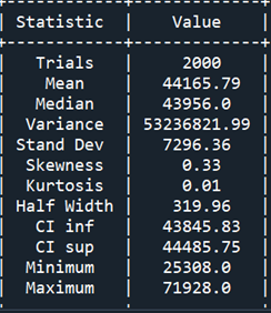
Desk 1 reveals little distinction between the imply and the median and the half-width interval is sort of negligible. The result distribution is positively skewed with a negligible diploma of kurtosis.
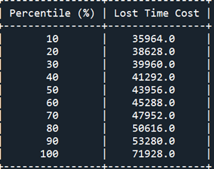
Desk 2 reveals the Percentile Report. We will see that the prospect that the misplaced time value will probably be better than 50 M U$S is greater than 20%.
Determine 1 reveals the distribution of our end result (Misplaced Time Value) as a histogram with 20 bins. The imply and the median are indicated with inexperienced and crimson vertical strains respectively. As typical, the histogram supplies a visible illustration of the distribution of our amount of curiosity: its location, unfold, skewness, and kurtosis. We declare that the anticipated worth (95% confidence degree) is round USS 44.000.
Determine 2 shows a density plot of the output variable % Misplaced Time. Keep in mind that the important thing concept in density plots is to eradicate the jaggedness that characterizes histograms, permitting higher visualization of the form of the distribution.
Clearly, the distribution is unimodal. We declare that, on common, 10% of the working hours will probably be misplaced resulting from machine breakdowns.
A Monte Carlo Simulation is a computational method utilized by decision-makers and challenge managers to quantitatively assess the affect of danger. An important step of any simulation research is an applicable statistical evaluation of the output knowledge. Statistical studies and distribution charts (histograms and density plots) are necessary for assessing the extent of publicity to danger.
