
With boosted determination tree algorithms, akin to XGBoost, CatBoost, and LightBoost chances are you’ll outperform different fashions however overfitting is an actual hazard. Discover ways to break up the info, optimize hyperparameters, and discover the best-performing mannequin with out overtraining it utilizing the HGBoost library.
Gradient boosting strategies gained a lot reputation lately for classification and regression duties. An essential half is the tuning of hyperparameters to achieve the most effective efficiency in predictions. This requires looking throughout 1000’s of parameter mixtures which isn’t solely a computationally-intensive activity however can rapidly result in overtrained fashions. Consequently, a mannequin could not generalize on new (unseen) information, and the efficiency accuracy might be worse than anticipated. Fortunately there are Bayesian optimization strategies that may assist to optimize the grid search and scale back the computational burden. However there’s extra to it as a result of an optimized grid search should still end in overtrained fashions. Fastidiously splitting your information right into a prepare set, a check set, and an unbiased validation set is one other essential half that must be integrated when optimizing hyperparameters. Right here comes the HGBoost library into play! HGBoost stands for Hyperoptimized Gradient Boosting and is a Python package deal for hyperparameter optimization for XGBoost, LightBoost, and CatBoost. It should rigorously break up the dataset right into a prepare, check, and unbiased validation set. Throughout the train-test set, there’s the inside loop for optimizing the hyperparameters utilizing Bayesian optimization (with hyperopt) and, the outer loop to attain how properly the highest performing fashions can generalize based mostly on k-fold cross validation. As such, it would make the most effective try to pick probably the most strong mannequin with the most effective efficiency. On this weblog, I’ll first briefly focus on boosting algorithms and hyperparameter optimization. Then I’ll soar into easy methods to prepare a mannequin with optimized hyperparameters. I’ll exhibit easy methods to interpret and visually clarify the optimized hyperparameter area and easy methods to consider the mannequin efficiency.
Gradient boosting algorithms akin to Excessive Gradient Boosting (XGboost), Gentle Gradient Boosting (Lightboost), and CatBoost are highly effective ensemble machine studying algorithms for predictive modeling that may be utilized on tabular and steady information, and for each classification and regression duties.
It isn’t shocking that boosted determination tree algorithms are highly regarded as a result of these algorithms had been concerned in additional than half of the successful options in machine studying challenges hosted at Kaggle [1]. It’s the mixture of gradient boosting with determination bushes that gives state-of-the-art leads to many purposes. It is usually this mixture that makes the distinction between the XGboost, CatBoost, and Lightboost. The widespread theme is that every boosting algorithm wants to seek out the most effective break up for every leaf, and desires to reduce the computational price. The excessive computational price is as a result of the mannequin wants to seek out the actual break up for every leaf, and that requires iterative scanning by means of all the info. This course of is difficult to optimize.
Roughly, there are two completely different methods to compute the bushes: level-wise and leaf-wise. The extent-wise technique grows the tree degree by degree. On this technique, every node splits the info and prioritizes the nodes nearer to the tree root. The leaf-wise technique grows the tree by splitting the info on the nodes with the very best loss change. Stage-wise development is normally higher for smaller datasets whereas leaf-wise tends to overfit in small datasets. Nevertheless, leaf-wise development tends to excel in bigger datasets the place it’s significantly sooner than level-wise development [2]. Let’s summarize the XGboost, LightBoost, and CatBoost algorithms when it comes to tree splitting, and computational prices.
XGBoost.
Excessive Gradient Boosting (XGboost) is among the hottest varieties of gradient boosting strategies for which the boosted determination bushes are internally made up of an ensemble of weak determination bushes. Initially XGBoost was based mostly on a level-wise development algorithm however just lately has added an possibility for leaf-wise development that implements break up approximation utilizing histograms. The benefits are that XGBoost is efficient in studying and has sturdy generalization efficiency. As well as, it will probably additionally seize nonlinear relationships. The disadvantages are that the hyperparameter tuning might be complicated, it doesn’t carry out properly on sparse datasets, and might rapidly end in excessive computational prices (each memory-wise and time-wise) as many bushes are wanted when utilizing very giant datasets [2].
LightBoost.
LightBoost or LightGBM is a gradient boosting framework that makes use of tree-based studying algorithms for which the bushes are break up vertically (or leaf-wise). Such an method might be extra environment friendly in loss discount in comparison with a level-wise algorithm when rising the identical leaf. As well as, LightBoost makes use of histogram-based algorithms, which buckets steady characteristic values into discrete bins. This accelerates coaching and reduces reminiscence utilization. It’s designed to be environment friendly and has many benefits, akin to quick coaching, excessive effectivity, low reminiscence utilization, higher accuracy, help of parallel and GPU studying, and functionality of dealing with large-scale information [3]. The computation and reminiscence environment friendly benefits make LightBoost relevant for giant quantities of information. The disadvantages are that it’s delicate to overfitting because of leaf-wise splitting, and excessive complexity because of hyperparameter tuning.
CatBoost.
CatBoost can also be a high-performance methodology for gradient boosting on determination bushes. Catboost grows a balanced tree utilizing oblivious bushes or symmetric bushes for sooner execution. Which means that pér characteristic, the values are divided into buckets by creating feature-split pairs, akin to (temperature, <0), (temperature, 1–30), (temperature, >30), and so forth. In every degree of an oblivious tree, the feature-split pair that brings the bottom loss (in line with a penalty operate) is chosen and is used for all the extent nodes. It’s described that CatBoost supplies nice outcomes with default parameters and can due to this fact require much less time on parameter tuning [4]. One other benefit is that CatBoost permits you to use non-numeric elements, as an alternative of getting to pre-process your information or spend effort and time turning it into numbers [4]. A number of the disadvantages are: It must construct deep determination bushes to get better dependencies in information in case of options with excessive cardinality, and it doesn’t work with lacking values.
Every boosted determination tree has its personal (dis)benefits and due to this fact you will need to have a great understanding of the dataset you might be working with together with the appliance you goal to develop.
Just a few phrases in regards to the definition of hyperparameters, and the way they differ from regular parameters. Total we are able to say that regular parameter are optimized by the machine studying mannequin itself whereas hyperparameters will not be. Within the case of a regression mannequin, the connection between the enter options and the result (or goal worth) is realized. Throughout the coaching of the regression mannequin, the slope of the regression line is optimized by tuning the weights (beneath the belief that the connection with the goal worth is linear). Or in different phrases, the mannequin parameters are realized throughout the coaching part.
Parameters are optimized by the machine studying mannequin itself, whereas hyperparameters are exterior the coaching course of and require a meta-process for tuning.
Then there’s one other set of parameters often known as hyperparameters, (additionally named as nuisance parameters in statistics). These values should be specified exterior of the coaching process and are the enter parameters for the mannequin. Some fashions shouldn’t have any hyperparameters, others have a couple of (two or three or so) that may nonetheless be manually evaluated. Then there are fashions with a number of hyperparameters. I imply, actually loads. Boosted determination tree algorithms, akin to XGBoost, CatBoost, and LightBoost are examples which have a number of hyperparameters, consider desired depth, variety of leaves within the tree, and so forth. You could possibly use the default hyperparameters to coach a mannequin however tuning the hyperparameters typically results in a huge impact on the ultimate prediction accuracy of the educated mannequin [8]. As well as, completely different datasets require completely different hyperparameters. That is troubling as a result of a mannequin can simply comprise tens of hyperparameters, which subsequently can lead to (tens of) 1000’s of hyperparameter mixtures that should be evaluated to find out the mannequin efficiency. That is known as the search area. The computational burden (time-wise and memory-wise) can due to this fact be monumental. Optimizing the search area is thus useful.
For supervised machine studying duties, you will need to break up the info into separate components to keep away from overfitting when studying the mannequin. Overfitting is when the mannequin suits (or learns) on the info too properly after which fails to foretell (new) unseen information. The commonest method is to separate the dataset right into a prepare set, and an unbiased validation set. Nevertheless, once we additionally carry out hyperparameter tuning, akin to in boosting algorithms, it additionally requires a check set. The mannequin can now see the info, study from the info, and at last, we are able to consider the mannequin on unseen information. Such an method doesn’t solely prevents overfitting but additionally helps to find out the robustness of the mannequin i.e., with a okay-fold cross-validation method. Thus when we have to tune hyperparameters, we must always separate the info into three components, specifically: prepare set, check set, and validation set.
- The Prepare set: That is the half the place the mannequin sees and learns from the info. It consists usually 70% or 80% of the samples to find out the most effective match throughout the 1000’s of attainable hyperparameters (e.g., utilizing a okay-fold-cross validation scheme).
- The check set: This set incorporates usually 20% of the samples, and can be utilized to judge the mannequin efficiency, akin to for the precise set of hyperparameters.
- The validation set: This set additionally incorporates usually 20% of the samples within the information however is saved untouched till the very last mannequin is educated. The mannequin can now be evaluated in an unbiased method. You will need to notice that this set can solely be used as soon as. Or in different phrases, if the mannequin is additional optimized after getting insights on the validation set, you want one other unbiased set to find out the final-final mannequin efficiency.
Establishing a nested cross-validation method might be time-consuming and even a sophisticated activity, however crucial in case you wish to create a sturdy mannequin, and stop overfitting. It’s a good train to make such an method your self, however these are additionally applied within the HGBoost library [1]. Earlier than I’ll focus on the working of HGBoost, I’ll first briefly describe the Bayesian method for large-scale optimization of fashions with completely different hyperparameter mixtures.
When utilizing boosted determination tree algorithms, there can simply be tens of enter hyperparameters which might subsequently result in (tens of) 1000’s of hyperparameter mixture that must be evaluated. This is a vital activity as a result of a particular mixture of hyperparameters can lead to extra correct predictions for the precise dataset. Though there are numerous hyperparameters to tune, some are extra essential than others. Furthermore, some hyperparameters can have little or no impact on the result however with no good method, all mixtures of hyperparameters should be evaluated to seek out the most effective performing mannequin. This makes it a computational burden.
Hyperparameter optimization could make an enormous distinction within the accuracy of a machine studying mannequin.
Looking throughout mixtures of parameters is commonly carried out with grid searches. Basically, there are two varieties: grid search and random search which can be utilized for parameter tuning. Grid search will iterate throughout your complete search area and is thus very efficient but additionally very-very sluggish. However, a random search is quick as it would randomly iterate throughout the search area, and whereas this method has been confirmed to be efficient, it might simply miss a very powerful factors within the search area. Fortunately, a 3rd possibility exists: sequential model-based optimization, often known as Bayesian optimization.
Bayesian optimization for parameter tuning is to find out the most effective set of hyperparameters inside a number of iterations. The Bayesian optimization method is an environment friendly methodology of operate minimization and is applied within the Hyperopt library. The effectivity makes it applicable for optimizing the hyperparameters of machine studying algorithms which are sluggish to coach [5]. In-depth particulars about Hyperopt might be discovered on this weblog [6]. To summarize, it begins by sampling random mixtures of parameters and computes the efficiency utilizing a cross-validation scheme. Throughout every iteration, the pattern distribution is up to date and in such a fashion, it turns into extra prone to pattern parameter mixtures with a great efficiency. An important comparability between the normal grid search, random search, and Hyperopt might be discovered on this weblog.
The effectivity of Bayesian optimization makes it applicable for optimizing the hyperparameters of machine studying algorithms which are sluggish to coach [5].
Hyperopt is integrated into the HGBoost method to do the hyperparameter optimization. Within the subsequent part, I’ll describe how the completely different components of splitting the dataset and hyperparameter optimization are taken care of, which incorporates the target operate, the search area, and the analysis of all trials
The Hyperoptimized Gradient Boosting library (HGBoost), is a Python package deal for hyperparameter optimization for XGBoost, LightBoost, and CatBoost. It should break up the dataset right into a prepare, check, and unbiased validation set. Throughout the train-test set, there’s the inside loop for optimizing the hyperparameters utilizing Bayesian optimization (utilizing hyperopt) and, the outer loop to attain how properly the best-performing fashions can generalize utilizing okay-fold cross validation. Such an method has the benefit of not solely choosing the mannequin with the very best accuracy but additionally the mannequin that may finest generalize.
HGBoost has many benefits, akin to; it makes the most effective try and detect the mannequin that may finest generalize, and thereby decreasing the opportunity of choosing an overtrained mannequin. It supplies explainable outcomes by offering insightful plots akin to; a deep examination of the hyperparameter area, the efficiency of all evaluated fashions, the accuracy for the k-fold cross-validation, the validation set, and final however not least the most effective determination tree might be plotted along with a very powerful options.
What advantages does hgboost provide extra:
- It consists of the most well-liked determination tree algorithms; XGBoost, LightBoost, and Catboost.
- It consists of the most well-liked hyperparameter optimization library for Bayesian Optimization; Hyperopt.
- An automatic method to separate the dataset right into a train-test and unbiased validation to attain the mannequin efficiency.
- The pipeline has a nested scheme with an inside loop for hyperparameter optimization and an outer loop with okay-fold cross-validation to find out probably the most strong and best-performing mannequin.
- It will probably deal with classification and regression duties.
- It’s simple to go wild and create a multi-class mannequin or an ensemble of boosted determination tree fashions.
- It takes care of unbalanced datasets.
- It creates explainable outcomes for the hyperparameter search-space, and mannequin efficiency outcomes by creating insightful plots.
- It’s open-source.
- It’s documented with many examples.
The HGBoost method consists of varied steps within the pipeline. The schematic overview is depicted in Determine 1. Let’s undergo the steps.

Step one is to separate the dataset into the coaching set, a testing set, and, an unbiased validation set. Understand that the validation set is saved untouched throughout your complete coaching course of and used on the very finish to judge the mannequin efficiency. Throughout the train-test set (Determine 1A), there’s the inside loop for optimizing the hyperparameters utilizing Bayesian optimization and, the outer loop to check how properly the best-performing fashions can generalize on unseen check units utilizing exterior okay-fold cross validation. The search area is dependent upon the out there hyperparameters of the mannequin kind. The mannequin hyperparameters that wants optimization are proven in code part 1.
Within the Bayesian optimization half, we reduce the price operate over a hyperparameter area by exploring your complete area. In contrast to a conventional grid search, the Bayesian method searches for the most effective set of parameters and optimizes the search area after every iteration. The fashions are internally evaluated utilizing a okay-fold cross-validation method. Or in different phrases, we are able to consider a hard and fast variety of operate evaluations, and take the most effective trial. The default is about to 250 evaluations which thus leads to 250 fashions. After this step, you may now take the best-performing mannequin (based mostly on the AUC or every other metric) after which cease. Nevertheless, that is strongly discouraged as a result of we simply searched all through your complete search area for a set of parameters that now appears to suit the most effective on the coaching information, with out figuring out how properly it generalizes. Or in different phrases, the best-performing mannequin could or-may-not be overtrained. To keep away from discovering an overtrained mannequin, the k-fold cross-validation scheme will proceed our quest to seek out probably the most strong mannequin. Let’s go to the second step.
The second step is rating the fashions (250 on this instance) on the desired analysis metric (the default is about to AUC), after which taking the highest p finest performing fashions (default is about to p=10). In such a fashion, we don’t depend on a single mannequin with the most effective hyperparameters that may-or-may-not be overfitted. Be aware that every one 250 fashions might be evaluated however that is computationally intensive and due to this fact we take the most effective p(erforming) fashions. To find out how the highest 10 performing fashions generalize, a okay-fold cross-validation scheme is used for the analysis. The default for okay is 5 folds, which signifies that for every of the p fashions, we are going to look at the efficiency throughout the okay=5 folds. To make sure the cross-validation outcomes are comparable between the highest p=10 fashions, sampling is carried out in a stratified method. In whole, we are going to consider p x okay; 10×5=50 fashions.
Within the third step, we’ve the p finest performing fashions, and we computed their efficiency in a okay-fold cross-validation method. We will now compute the typical accuracy (e.g., AUC) throughout the okay-folds, then rank the fashions, and at last choose the very best ranked mannequin. The cross-validation method will assist to pick probably the most strong mannequin, i.e., the one that may additionally generalize throughout completely different units of information. Be aware that different fashions could exist that end in higher efficiency with out the cross-validation method however these could also be overtrained.
Within the fourth step, we are going to look at the mannequin accuracy on the unbiased validation set. This set has been untouched to date and can due to this fact give a great estimate. Due to our intensive mannequin choice method (whether or not the mannequin can generalize, and restrict the likelihood to pick an overtrained mannequin), we must always not count on to giant variations in efficiency in comparison with our readily seen outcomes.
Within the very last step, we are able to re-train the mannequin utilizing the optimized parameters on your complete dataset (Determine 1C). The following step (Determine 1D) is the interpretation of the outcomes for which insightful plots might be created.
Earlier than we are able to use HGBoost, we have to set up it first utilizing the command line:
pip set up hgboost
After the set up, we are able to import HGBoost and initialize. We will maintain the enter parameters to their defaults (depicted in code part 2) or change them accordingly. Within the subsequent sections, we are going to undergo the set of parameters.
The initialization is saved constant for every activity (classification, regression, multi-class, or ensemble), and every mannequin (XGBoost, LightBoost, and CatBoost) which makes it very simple to modify between the completely different determination tree fashions and even duties. The output can also be saved constant which is a dictionary that incorporates six keys as proven in code part 3.
For demonstration, let’s use the Titanic dataset [10] that may be imported utilizing the operate import_example(information=’titanic’). This information set is freed from use and was a part of the Kaggle competitors Machine Studying from Catastrophe. The preprocessing step might be carried out utilizing the operate .preprocessing() which depends on the df2onehot library [11]. This operate will encode the specific values into one-hot and maintain the continual values untouched. I manually eliminated some options, akin to PassengerId and Identify (code part 4). Be aware that in regular use-cases, it is suggested to rigorously do the Exploratory Information Evaluation, characteristic cleansing, characteristic engineering, and so forth. The most important efficiency beneficial properties usually observe from these first steps.
Understand that the preprocessing steps could differ when coaching a mannequin with XGBoost, LightBoost, or CatBoost. For example, does the mannequin require encoding of the options or can it deal with non-numeric options? Can the mannequin deal with lacking values or ought to the options be eliminated? See part A really temporary introduction to Boosting Algorithms to learn extra particulars in regards to the (dis)benefits between the three fashions and do the preprocessing accordingly.
Prepare a Mannequin.
After initialization, we are able to use the XGBoost determination tree to coach a mannequin. Be aware that you would be able to additionally use the LightBoost or CatBoost mannequin as proven in code part 3. Throughout the coaching course of (operating the code in part 4), it would iterate throughout the search area and create 250 completely different fashions (max_eval=250) for which the mannequin accuracy is evaluated for the set of hyperparameters which are out there for the actual determination tree mannequin (XGBoost on this case, code part 1). Subsequent, the fashions are ranked on their accuracy, and the highest 10 best-performing fashions are chosen top_cv_evals=10. These are actually additional investigated utilizing the 5 fold cross-validation scheme (cv=5) to attain how properly the fashions generalize. On this sense, we goal to forestall discovering an overtrained mannequin.
All examined hyperparameters for the completely different fashions are returned which might be additional examined (manually) or through the use of the plot performance. For example, the output of HGBoost is depicted in code part 5 and extra particulars in Determine 2.

After the ultimate mannequin is returned, varied plots might be created for a deeper examination of the mannequin efficiency and the hyperparameter search area. This may also help to achieve higher instinct and explainable outcomes on how the mannequin parameters behave in relation to the efficiency. The next plots might be created:
- to deeper examine the hyperparameter area.
- to summarize all evaluated fashions.
- to point out the efficiency utilizing the cross-validation scheme.
- the outcomes on the unbiased validation set.
- The choice tree plot for the most effective mannequin and the most effective performing options.
Interpretation of the Hyperparameter Tuning.
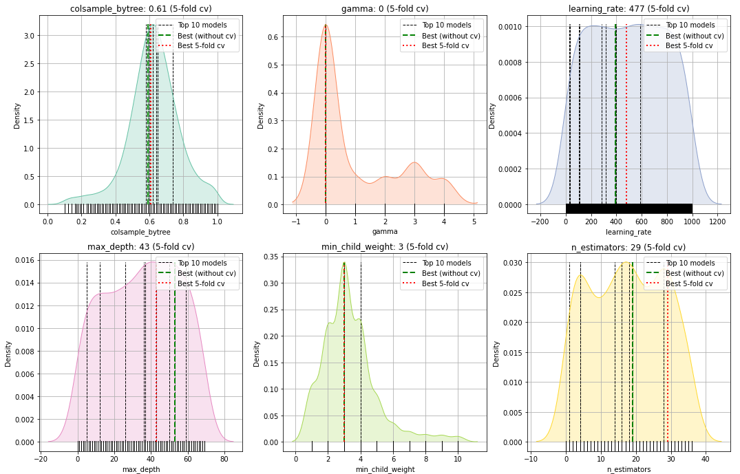
To deeper examine the hyperparameter area, the operate .plot_params() can be utilized (Determine 3 and 4). Let’s begin by investigating how the hyperparameters are tuned throughout the Bayesian Optimization course of. Each figures comprise a number of histograms (or kernel density plots), the place every subplot is a single parameter that’s optimized throughout the 250 mannequin iterations. The small bars on the backside of the histogram depict the 250 evaluations, whereas the black dashed vertical strains depict the precise parameter worth that’s used throughout the highest 10 best-performing fashions. The inexperienced dashed line depicts the best-performing mannequin with out the cross-validation method, and the pink dashed line depicts the best-performing mannequin with cross-validation.
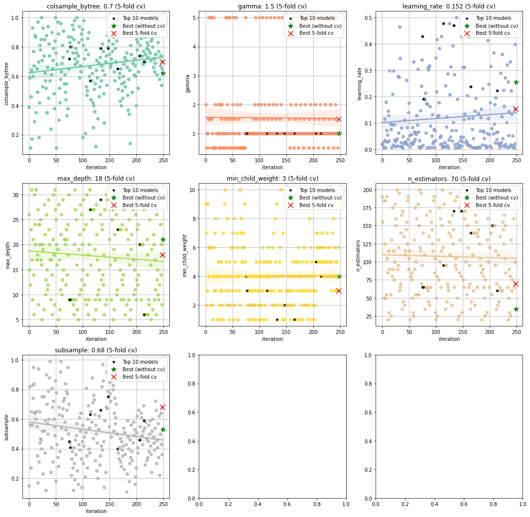
Let’s take a look at Determine 3. On the left prime nook, there’s the parameter colsample_bytree for which the values are chosen within the vary from 0 as much as 1.2. The typical worth for colsample_bytree is ~0.7 which signifies that the optimized pattern distribution utilizing the Bayesian optimization for this parameter has moved to this worth. Our greatest-performing mannequin has the worth of precisely colsample_bytree=0.7, (pink dashed line). However there’s extra to have a look at. Once we now have a look at Determine 4, we even have the colsample_bytree for which every dot is among the 250 fashions sorted on the iteration quantity. The horizontal axes are the iterations and the vertical axis are optimized parameter values. For this parameter, there’s an upwards pattern throughout the iterations of the optimization course of; in direction of the worth of 0.7. This means that throughout the iterations, the search area for colsample_bytree was optimized and extra fashions had been seen with higher accuracy when growing the worth of colsample_bytree. On this method, all of the hyperparameters might be interpreted in relation to the completely different fashions.

Interpretation of the mannequin efficiency throughout all evaluated fashions.
With the plot operate .plot() we are able to get insights into the efficiency (AUC on this case) of the 250 fashions (Determine 4). Right here once more, the inexperienced dashed line depicts the best-performing mannequin with out the cross-validation method, and the pink dashed line depicts the best-performing mannequin with cross-validation. Determine 5 depicts the ROC curve for the best-performing mannequin with optimized hyperparameters in comparison with a mannequin with default parameters.


Resolution Tree plot of the most effective mannequin.
With the choice tree plot (Determine 6) we are able to get a greater understanding of how the mannequin works. It might additionally give some instinct whether or not such a mannequin can generalize over different datasets. Be aware that the most effective tree is returned by default num_tree=0however many bushes are created that may be returned by specifying the enter parameter .treeplot(num_trees=1) . As well as, we are able to additionally plot the best-performing options (not proven right here).

Make Predictions.
After having the ultimate educated mannequin, we are able to now use it to make prediction on new information. Suppose that X is new information, and is equally pre-processed as within the coaching course of, then we are able to use the .predict(X) operate to make predictions. This operate returns the classification chance and the prediction label. See code part 7 for an instance.
Save and cargo mannequin.
Saving and loading fashions can turn out to be useful. With a view to accomplish this, there are two capabilities: .save() and performance .load()(code part 8).
I demonstrated easy methods to prepare a mannequin with optimized hyperparameters by splitting the dataset right into a prepare, check, and unbiased validation set. Throughout the train-test set, there’s the inside loop for optimizing the hyperparameters utilizing Bayesian optimization, and the outer loop to attain how properly the highest performing fashions can generalize based mostly on k-fold cross validation. On this method, we make the most effective try to pick the mannequin that may generalize and with the most effective accuracy.
An essential half earlier than coaching any mannequin is to do the standard modeling workflow: first do the Exploratory Information Evaluation (EDA), iteratively do the cleansing, characteristic engineering, and have choice. The most important efficiency beneficial properties usually observe from these steps.
HGBoost helps studying classification fashions, regression fashions, multi-class fashions, and even an ensemble of boosting tree fashions. For all duties, the identical process is utilized to ensure the best-performing and most strong mannequin is chosen. Moreover, it depends on HyperOpt to do the Bayesian optimization which is among the hottest libraries for hyperparameter optimization. One other Bayesian optimization algorithm that’s just lately developed is known as Optuna. In case you wish to learn extra particulars, and a comparability between the 2 strategies, strive this weblog.
That is it. I hope you loved studying it! Let me know if one thing shouldn’t be clear or when you’ve got every other solutions.
Be secure. Keep frosty.
Cheers, E.
- Nan Zhu et al, XGBoost: Implementing the Winningest Kaggle Algorithm in Spark and Flink.
- Miguel Fierro et al, Classes Realized From Benchmarking Quick Machine Studying Algorithms.
- Welcome to LightGBM’s documentation!
- CatBoost is a high-performance open supply library for gradient boosting on determination bushes.
- James Bergstra et al, 2013, Hyperopt: A Python Library for Optimizing the Hyperparameters of Machine Studying Algorithms.
- Kris Wright, 2017, Parameter Tuning with Hyperopt.
- E.Taskesen, 2019, Classeval: Analysis of supervised predictions for two-class and multi-class classifiers.
- Alice Zheng, Chapter 4. Hyperparameter Tuning.
- E. Taskesen, 2020, Hyperoptimized Gradient Boosting.
- Kaggle, Machine Studying from Catastrophe.
- E.Taskesen, 2019, df2onehot: Convert unstructured DataFrames into structured dataframes.
