
Every thing about Knowledge Transformation, Polynomial Regression, and Nonlinear Regression

A Easy linear regression (SLR) mannequin is straightforward to assemble when the connection between the goal variable and the predictor variables is linear. When there’s a nonlinear relationship between a dependent variable and impartial variables, issues turn out to be extra sophisticated. On this article, I’ll present you three totally different approaches to constructing a regression mannequin on the identical nonlinear dataset:
1. Polynomial regression
2. Knowledge transformation
3. Nonlinear regression
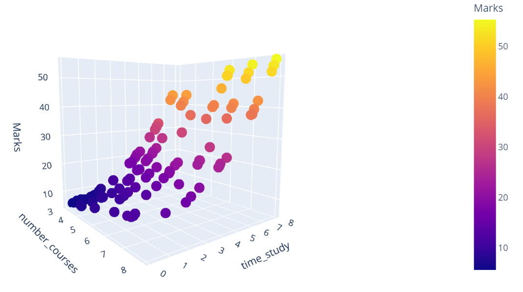
The dataset that I’ve thought of has been taken from Kaggle: https://www.kaggle.com/datasets/yasserh/student-marks-dataset
The info consists of Marks of scholars together with their examine time & variety of programs.

In case you look at the relationships of the goal variables “Marks” w.r.to review time and variety of programs, you’ll find that the connection is non-linear.
I attempted to construct a linear regression mannequin utilizing sklearn LinearRegression() mannequin. I outlined a operate to calculate numerous metrics for the mannequin.
and after I referred to as this operate for my mannequin, I bought the beneath output.
R2-Sq. Worth: 0.94
RSS: 1211.696
MSE: 12.117
EMSE: 3.481
94% r2-score isn’t unhealthy, however we are going to shortly see that this will get higher with a non-linear regression mannequin. The issue is extra with the assumptions behind the linear regression mannequin.
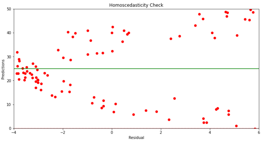
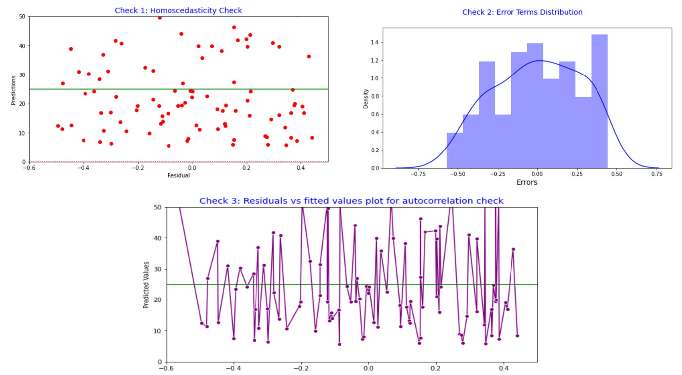
SLR Assumption 1: Homoscedasticity
Homoscedasticity signifies that the residuals have equal or nearly equal variance throughout the regression line. By plotting the error phrases with predicted phrases we should always affirm that there isn’t a sample within the error phrases. Nevertheless, on this case, we are able to clearly see that error phrases has a sure form.
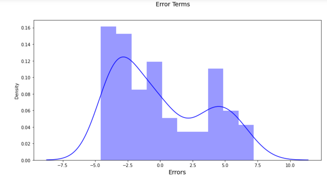
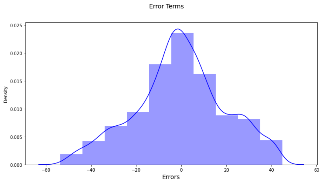
SLR Assumption 2: Error phrases are usually distributed
A bell-shaped distribution with a standard or almost regular distribution ought to ideally be seen for the error phrases. Nevertheless, from the graph beneath, it’s clear that we’ve a bi-model distribution. Consequently, on this case, the assumptions of linear regression have been damaged.
SLR Assumption 3: Error phrases are impartial of one another
The auto-correlation between error phrases ought to due to this fact not exist. Nevertheless, the figures beneath reveal that the error phrases seem to exhibit a point of auto-correlation.

Thus far, Now we have verified that the info is nonlinear, but we nonetheless construct an SLR equation. Though we achieved a good r2-score of 94%, not one of the SLR assumptions are met. SLR is due to this fact not a smart resolution for this kind of knowledge. We are going to now examine different methods for bettering the mannequin on the identical dataset.
Non-linear regressions are a relationship between impartial variables x and a dependent variable y which lead to a non-linear operate modeled knowledge. Basically any relationship that isn’t linear will be termed as non-linear, and is normally represented by the polynomial of ok levels (most energy of x).
y = a x³ + b x² + c x + d
Non-linear capabilities can have parts like exponentials, logarithms, fractions, and others. For instance: y = log(x)
And even, extra sophisticated reminiscent of :
y = log(a x³ + b x² + c x + d)
However what occurs if we’ve multiple impartial variables?
For two predictors, the equation of the polynomial regression turns into:

the place,
– Y is the goal,
– x1, x2 are the predictors or impartial variables
– 𝜃0 is the bias,
– and, 𝜃1, 𝜃2, 𝜃3, 𝜃4, and 𝜃5 are the weights within the regression equation
For n predictors, the equation covers all possible mixtures of assorted order polynomials. This is called Multi-dimensional Polynomial Regression and is notoriously tough to implement. We are going to assemble polynomial fashions of various levels and consider their efficiency. However first, let’s put together the dataset for coaching.
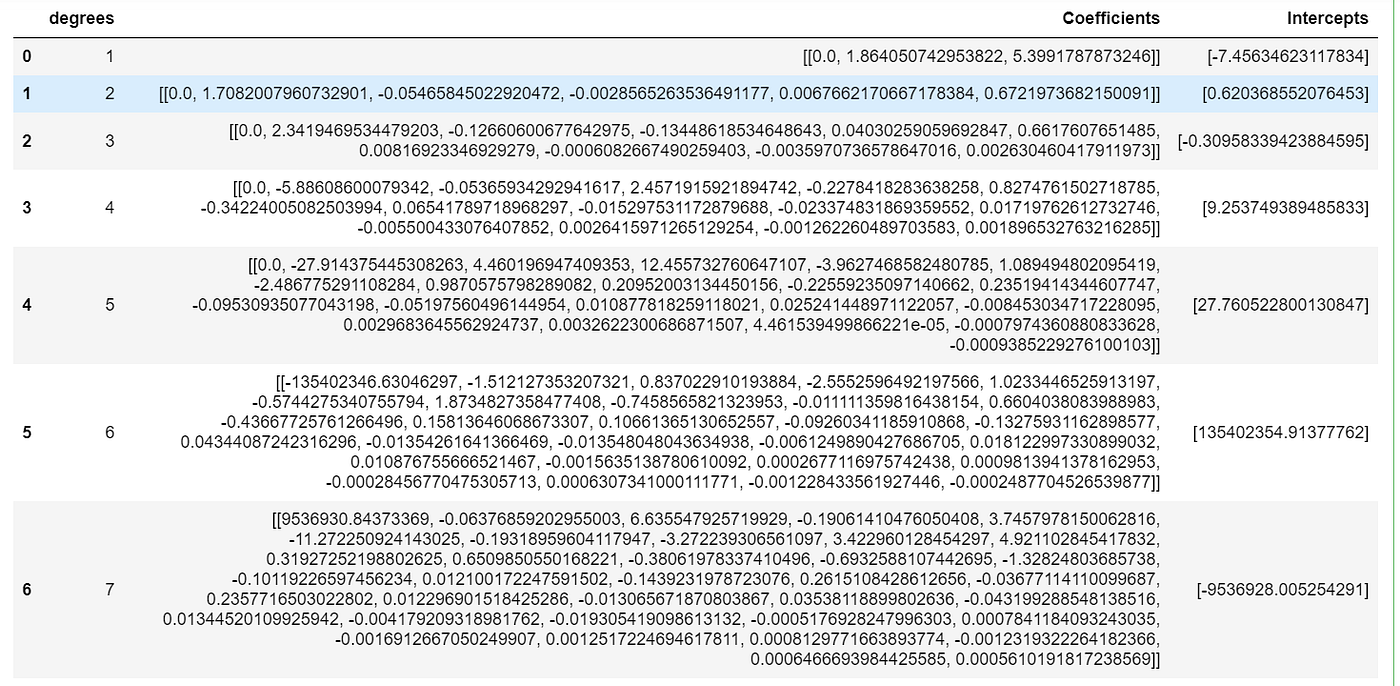
We are able to set up a pipeline and move the diploma and sophistication of fashions that we want to make the most of to provide a polynomial of assorted levels. That is what the code beneath does for us:
In case you want to view all the coefficients and intercepts, use the next code block: Please remember the fact that the variety of coefficients will fluctuate relying on the diploma of polynomial:
And right here is the output:
This doesn’t give a lot data on the efficiency of every mannequin, so will verify r2 rating.

So, we constructed polynomial equations as much as diploma 7 utilizing sklearn pipeline technique and located that diploma 2 and above yielded 99.9% accuracy (as in comparison with ~ 94% by SLR). On the identical dataset, we are going to now see one other approach for constructing a regression mannequin.
The linear regression framework assumes that the connection between the response and predictor variables is linear. To proceed using the linear regression framework, we’ve to change the info in order that the connection between variables turned linear.
Some Tips for knowledge transformations:
- Each the response and the predictor variables will be remodeled
- If the residual plot reveals the presence of nonlinear relationships within the knowledge, a simple technique is to make the most of nonlinear transformations of the predictors. In SLR, these transformations will be log(x), sqrt(x), exp(x), reciprocal, and so forth.
- It’s vital that every regressor have a linear reference to the goal variables. The transformation of dependent variables is one technique for addressing the non-linearity challenge.
In brief, normally:
- – Remodeling the y-values aids in coping with error phrases and should assist in non-linearity.
- The non-linearity is generally mounted by remodeling the x-values.
- For additional data on knowledge transformation, see https://on-line.stat.psu.edu/stat462/node/155/.
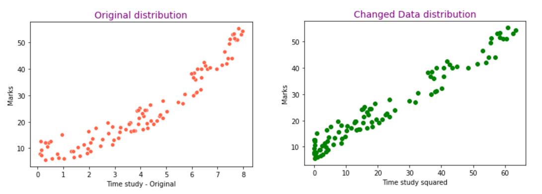
In our dataset, once we plotted the dependent variables “Marks” towards “time of examine” and “ variety of programs”, we noticed that Marks has non-linear relationship with time of examine. Therefore, we are going to do a metamorphosis on the characteristic time of examine.

After making use of the above transformation, we are able to plot Marks towards new characteristic time_study_sqaured to see if the connection has modified to linear.
Our dataset is now prepared for constructing a SLR mannequin. On this transformed dataset, we are going to now create a easy linear regression mannequin with the sklearn LinearRegression() technique. After we print the metrics after constructing the mannequin, we get the next end result:
R2-Sq. Worth: 0.9996
RSS: 7.083
MSE: 0.071
EMSE: 0.266
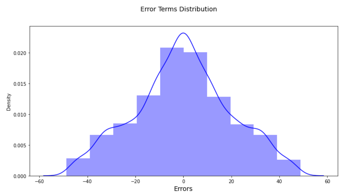
A big enchancment over the beforehand constructed SLR mannequin on the uncooked dataset (with none knowledge transformation). We bought a R2-Sq. Worth of 99.9% versus 94%. Now, we’ll validate the assorted assumptions of an SLR mannequin to see if it’s an excellent match.
So On this part, we remodeled the info itself. Understanding that characteristic time_study isn’t linearly dependent with Marks, we created a brand new characteristic referred to as time_study_squared, which was linearly dependent with Marks. Then we constructed a SLR mannequin once more and validated all of the assumptions of a SLR mannequin. We noticed that every one the assumptions are happy by this new mannequin. Now, it’s time to discover our subsequent and final methods to construct a distinct mannequin on the identical dataset.
For non-linear regression downside, we are able to strive SVR(), KNeighborsRegressor() or DecisionTreeRegression() from sklearn library, and examine the mannequin efficiency. Right here, we are going to develop our non-linear mannequin utilizing the sklearn SVR() approach for demonstration functions. SVR helps a wide range of Kernels. Kernels allow the linear SVM mannequin to separate nonlinearly separable knowledge factors. We are going to check three different kernels with the SVR algorithm and observe how they have an effect on mannequin accuracy:
- rbf (default kernal for SVR)
- linear
- poly
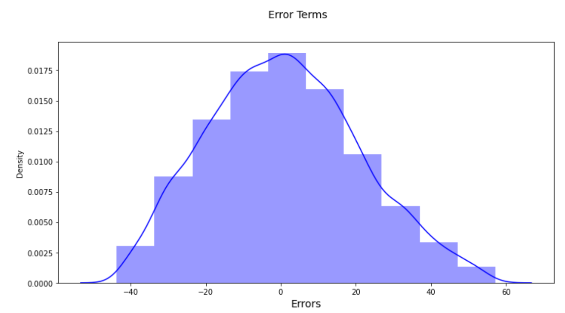
i. SVR() utilizing rbf kernal
And right here is the mannequin metrics: Nonetheless a greater R2-squared examine to our first SLR mannequin.
R2-Sq. Worth: 0.9982
RSS: 4053558.081
MSE: 0.363
EMSE: 0.602
A fast verify on the error time period distribution additionally appears to be OK.
ii. SVR() utilizing linear kernel
And right here is the mannequin metrics once we used the linear kernel: The R2-squared values once more dropped to ~93%
R2-Sq. Worth: 0.9350
RSS: 4063556.3
MSE: 13.201
EMSE: 3.633
And on this case additionally, error phrases appear to be a close to nor mal distribution curve:
iii. SVR() utilizing poly kernel
And listed here are the mannequin metrics with SVR poly kernel : The R2-squared worth is 97%, which is larger than the linear kernel however decrease than the rbf kernel.
R2-Sq. Worth: 0.9798
RSS: 4000635.359
MSE: 4.087
EMSE: 2.022
And right here is the error phrases distributions:
So, On this part, we created a non-linear mannequin utilizing sklearn SVR Mannequin with 3 totally different kernels. We bought one of the best R2-squared worth whith rbf kernel.
- r2-score with rbf kernel = 99.82%
- r2-score with linear kernel = 93.50 %
- r2-score with poly kernel = 97.98 %
On this submit, we began with a dataset that was not linearly depending on the goal variable. Earlier than we might examine different methods for constructing a regression mannequin on a non-linear dataset, we constructed a easy linear regression mannequin with a r2-score of 94%. We then investigated three distinct strategies for modelling a nonlinear dataset: Polynomial Regression, Knowledge Transformations, and a nonlinear regression mannequin (SVR). We found that polynomial levels of two and better resulted in a 99.9% r2-score, whereas SVR with a rbf kernel resulted in a 99.82% r2-score. Basically, at any time when we’ve a nonlinear dataset, we should always experiment with a number of methods and see which of them work finest.
Discover the info set and code right here: https://github.com/kg-shambhu/Non-Linear-Regression-Mannequin
You may contact me on LinkedIn: https://www.linkedin.com/in/shambhukgupta/
