Geospatial Website-Choice Evaluation Utilizing Cosine Similarity | by Elliot Humphrey | Jul, 2022

Figuring out similarities between geographic areas primarily based on neighbourhood facilities

Location is paramount for companies that function bodily areas, the place it’s key to be positioned near your goal market.

This problem is commonly the case for franchises which can be increasing into new areas the place it is very important perceive the ‘match’ of a enterprise in a brand new space. The purpose of this text is to discover this concept in additional element, to guage the suitability of a brand new location for a franchise primarily based on the traits of areas the place current franchises are positioned.

To realize this we will likely be taking information from OpenStreetMap of a well-liked espresso store franchise in Seattle, to make use of details about the encompassing neighbourhood to establish new potential areas which can be related.

To method this job there are just a few steps that must be thought-about:

1. Discovering current franchise areas
2. Figuring out close by facilities round these areas (which we are going to assume offers us an concept concerning the neighbourhood)
3. Discovering new potential areas and their close by facilities (repeating steps 1 & 2)
4. Evaluating the similarity between potential and current areas

As this job is geospatial, utilizing OpenStreetMap and packages like OSMNX and Geopandas will likely be helpful.

Discovering current franchise areas

As talked about, we are going to use a well-liked espresso store franchise to outline the present areas of curiosity. Amassing this data is relatively easy utilizing OSMNX, the place we are able to outline the geographic place of curiosity. I’ve set the place of curiosity as Seattle (USA), and outlined the title of the franchise utilizing the title/model tag in OpenStreetMap.

import osmnx
place = 'Seattle, USA'
gdf = osmnx.geocode_to_gdf(place)#Getting the bounding field of the gdf
bounding = gdf.bounds
north, south, east, west = bounding.iloc[0,3], bounding.iloc[0,1], bounding.iloc[0,2], bounding.iloc[0,0]
location = gdf.geometry.unary_union#Discovering the factors inside the space polygon
level = osmnx.geometries_from_bbox(north, south, east, west, tags={brand_name : 'espresso store'})
level.set_crs(crs=4326)
level = level[point.geometry.within(location)]#Ensuring we're coping with factors
level['geometry'] = level['geometry'].apply(lambda x : x.centroid if kind(x) == Polygon else x)
level = level[point.geom_type != 'MultiPolygon']
level = level[point.geom_type != 'Polygon']

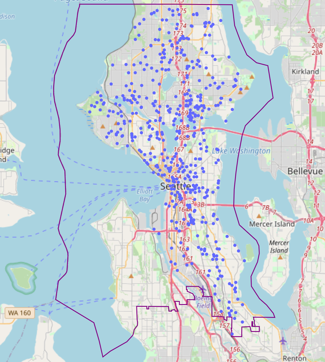
This offers us the areas of current franchise areas with our space:

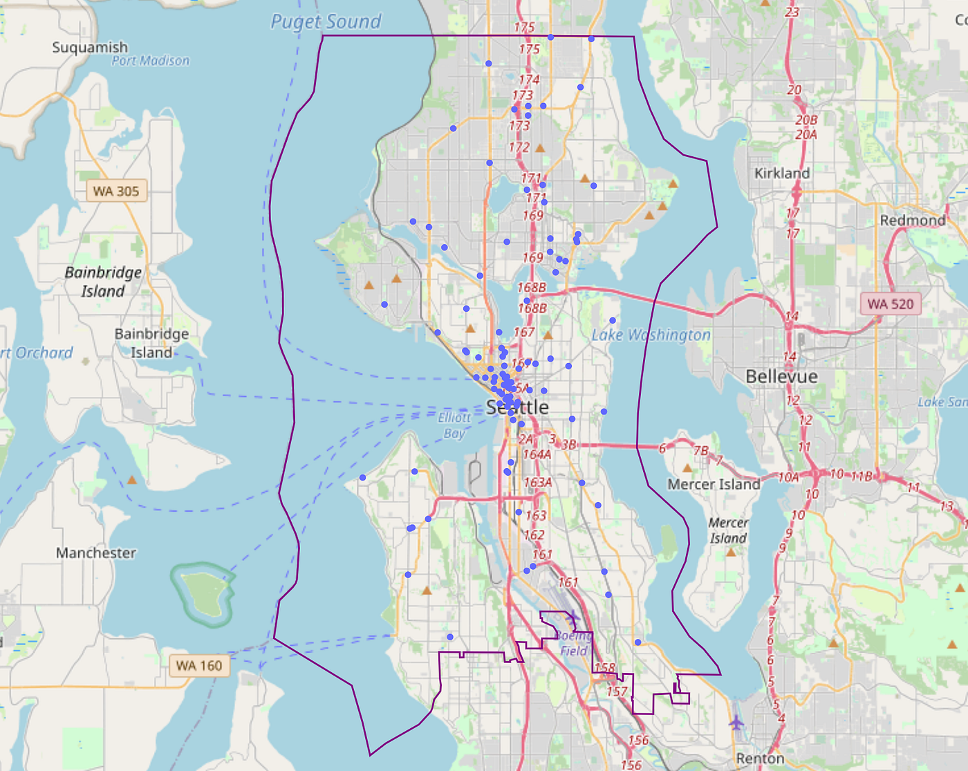
Trying on the current areas makes us marvel concerning the following:

1. What’s the density of the franchise on this areas?
2. What’s the spatial distribution of those areas (clustered shut collectively or evenly unfold out)?

To reply these questions we are able to calculate the franchise density utilizing the outlined space polygon and the rely of current franchises, which supplies us 0.262 per SqKm. Observe: giant areas within the polygon are water, due to this fact the density will seem a lot decrease right here than in actuality…

For measuring how dispersed these areas are relative to one another we are able to calculate the space to the closest neighbour utilizing Sklearn’s BallTree:

Nearest neighbours can be proven as a histogram:

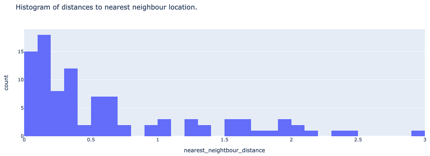
It seems like nearly all of areas exist with 800m of one another, which is clear when trying on the map and seeing the excessive density of current areas within the metropolis centre.

What concerning the facilities surrounding these areas?

We first have to get all of the facilities inside an space of curiosity and outline a radius round every current location, that can be utilized to establish close by facilities. This may be achieved utilizing one other BallTree, nonetheless querying factors primarily based on a specified radius (which I’ve set as 250m):

from sklearn.neighbors import BallTree#Defining the tree primarily based on lat/lon values transformed to radians
ball = BallTree(amenities_points[["lat_rad", "lon_rad"]].values, metric='haversine')#Querying the tree of facilities utilizing a radius round current areas
radius = ok / 6371000
indices = ball.query_radius(target_points[["lat_rad", "lon_rad"]], r = radius)
indices = pd.DataFrame(indices, columns={'indices'})

After we question OSM and use the BallTree to search out close by facilities we’re left with the indices of every amenity inside the radius of an current franchise location. Due to this fact we have to extract the amenity kind (e.g., restaurant) and rely every incidence to get a processed dataframe like the next:

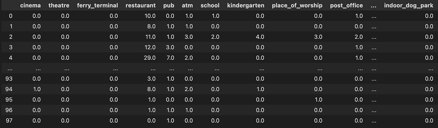
Now we are able to see the most well-liked facilities positioned close to current franchise areas in a sorted bar chart:

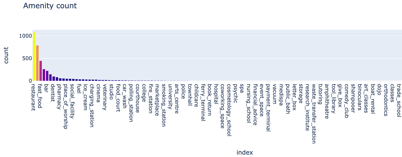
It seems that our espresso store franchise is dominantly positioned proximal to different areas that serve meals/drinks, together with just a few different minority facilities like ‘charging station’. This offers us the whole rely for all current areas, however are the distribution of facilities the identical?

We are able to apply fast PCA and DBSCAN clustering to see how current franchise areas cluster relative to one another (utilizing a min_sample worth of three):

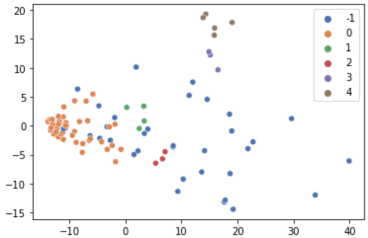
There’s a dominant cluster in the direction of the left, nonetheless different smaller clusters exist too. That is necessary because it tells us that current franchise areas fluctuate primarily based on their surrounding facilities and don’t conform to a single ‘kind’ of neighbourhood.

Now that now we have created a dataset for current franchise areas, we are able to now produce an analogous dataset for brand spanking new potential areas. We are able to randomly choose nodes that exist in our space of curiosity utilizing the graph extracted by OSMNX, as factors will likely be constrained to current paths accessible for strolling:

G = osmnx.graph_from_place(place, network_type='stroll', simplify=True)
nodes = pd.DataFrame(osmnx.graph_to_gdfs(G, edges=False)).pattern(n = 500, substitute = False)

Discovering close by facilities for every of those potential areas will be achieved by repeating the earlier steps…

Measuring the similarity between current and potential areas

That is the half we’ve been ready for; measuring the similarity between current and our potential areas. We’ll use the pairwise cosine similarity to attain this, the place every location consists of a vector primarily based on the variety and amount of facilities close by. Utilizing cosine similarity gives two advantages on this geospatial context:

1. Vector lengths don’t have to match = We are able to nonetheless measure similarities between areas with various kinds of facilities.
2. Similarity just isn’t primarily based on simply the frequency of facilities = Since we additionally care concerning the variety of facilities, not simply the magnitude.

We calculate the cosine similarity of a possible new location towards all different current areas, which signifies that now we have a number of similarity rating.

max_similarities = []
for j in vary(len(new_locations)):
similarity = []
for i in vary(len(existing_locations)):
cos_similarity = cosine_similarity(new_locations.iloc[[j]].values, existing_locations.iloc[[i]].values).tolist()
similarity.lengthen(cos_similarity)
similarity = [np.max(list(chain(*similarity)))]
average_similarities.lengthen(similarity)
node_amenities['averaged similarity score'] = max_similarities

So how will we outline what is comparable?

For this, we are able to do not forget that current areas don’t type a single cluster, which means there may be heterogeneity. A superb analogy will be when evaluating an individual can be part of a friendship group:

1. A friendship group usually will include completely different folks with various traits, and never a gaggle of individuals with similar traits.
2. Inside a gaggle, folks will share kind of traits with completely different members of the group.
3. A brand new potential member does not essentially must be much like everybody within the group to be thought-about match.

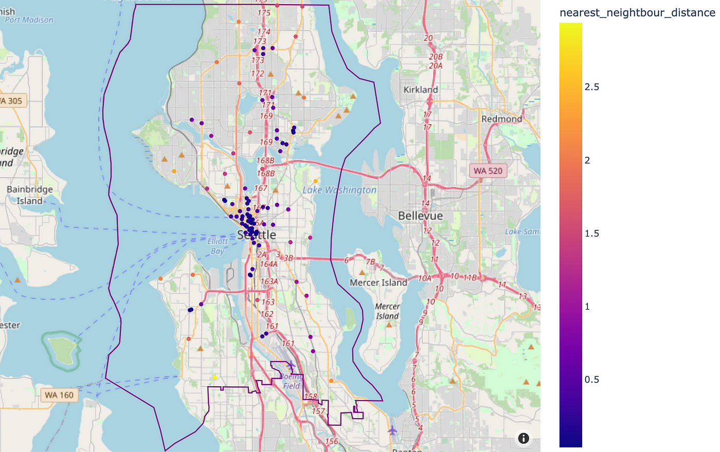
Due to this, we selected the most similarity rating when evaluating with current areas, as this tells us that the potential location is much like not less than one different current franchise location. Taking a median would result in decrease rating, since variation in close by facilities exists between franchise areas. We are able to now plot the outcomes, colored by similarity rating, to see what areas might be new franchise areas:

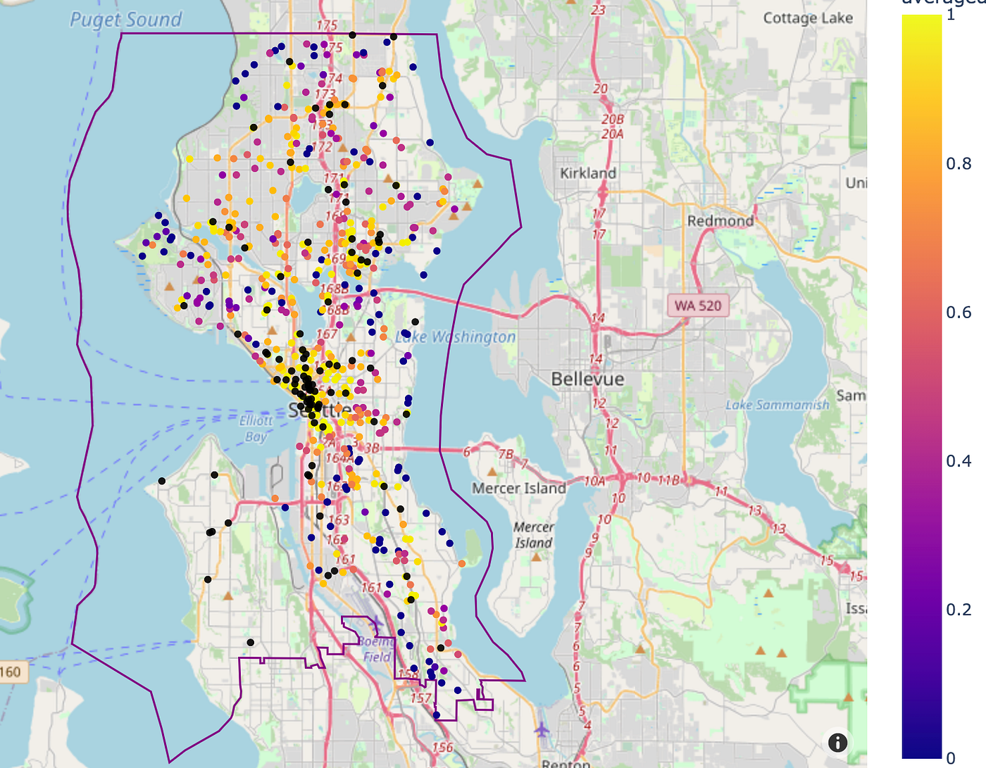
Our similarity scores for areas within the metropolis centre all present sturdy similarities with current areas, which is sensible, due to this fact what we’re actually curiosity in are the areas with excessive similarity scores which can be positioned far-off from current franchise areas (black factors on the map).

We’ve used geospatial strategies to guage the potential areas for a espresso store franchise to increase into new areas, utilizing cosine similarity scores primarily based on close by facilities. That is only a small piece of a much bigger image, the place components resembling inhabitants density, accessibility and so forth. must also be taken under consideration.

Preserve an eye fixed out for the subsequent article the place will begin to mature this concept additional with some modelling. Thanks for studying!