
An in depth information to one of the standard causal inference strategies within the trade

It’s now broadly accepted that the gold normal approach to compute the causal impact of a remedy (a drug, advert, product, …) on an end result of curiosity (a illness, agency income, buyer satisfaction, …) is AB testing, a.okay.a. randomized experiments. We randomly break up a set of topics (sufferers, customers, clients, …) right into a remedy and a management group and provides the remedy to the remedy group. This process ensures that ex-ante, the one anticipated distinction between the 2 teams is attributable to the remedy.
One of many key assumptions in AB testing is that there’s no contamination between the remedy and management group. Giving a drug to at least one affected person within the remedy group doesn’t have an effect on the well being of sufferers within the management group. This won’t be the case for instance if we are attempting to remedy a contagious illness and the 2 teams will not be remoted. Within the trade, frequent violations of the contamination assumption are community results — my utility of utilizing a social community will increase because the variety of associates on the community will increase — and common equilibrium results — if I enhance one product, it’d lower the gross sales of one other related product.
Due to this motive, usually experiments are carried out at a sufficiently massive scale in order that there isn’t any contamination throughout teams, reminiscent of cities, states, and even nations. Then one other downside arises due to the bigger scale: the remedy turns into dearer. Giving a drug to 50% of sufferers in a hospital is way inexpensive than giving a drug to 50% of cities in a rustic. Subsequently, usually solely a few items are handled however usually over an extended time period.
In these settings, a really highly effective methodology emerged round 10 years in the past: Artificial Management. The concept of artificial management is to take advantage of the temporal variation within the knowledge as an alternative of the cross-sectional one (throughout time as an alternative of throughout items). This methodology is extraordinarily standard within the trade — e.g. in corporations like Google, Uber, Fb, Microsoft, and Amazon — as a result of it’s simple to interpret and offers with a setting that emerges usually at massive scales. On this publish we’re going to discover this method by way of instance: we are going to examine the effectiveness of self-driving automobiles for a ride-sharing platform.
Suppose you had been a ride-sharing platform and also you needed to check the impact of self-driving automobiles in your fleet.
As you may think about, there are numerous limitations to working an AB/check for one of these characteristic. Initially, it’s difficult to randomize particular person rides. Second, it’s a really costly intervention. Third, and statistically most vital, you can not run this intervention on the trip stage. The issue is that there are spillover results from handled to manage items: if certainly self-driving automobiles are extra environment friendly, it implies that they will serve extra clients in the identical period of time, lowering the shoppers obtainable to regular drivers (the management group). This spillover contaminates the experiment and prevents a causal interpretation of the outcomes.
For all these causes, we choose just one metropolis. Given the artificial vibe of the article we can’t however choose… (drum roll)… Miami!

I generate a simulated dataset by which we observe a panel of U.S. cities over time. The income knowledge is made up, whereas the socio-economic variables are taken from the OECD 2022 Metropolitan Areas database. I import the information producing course of dgp_selfdriving() from src.dgp. I additionally import some plotting features and libraries from src.utils.
from src.utils import *
from src.dgp import dgp_selfdrivingtreatment_year = 2013
treated_city = 'Miami'
df = dgp_selfdriving().generate_data(yr=treatment_year, metropolis=treated_city)
df.head()
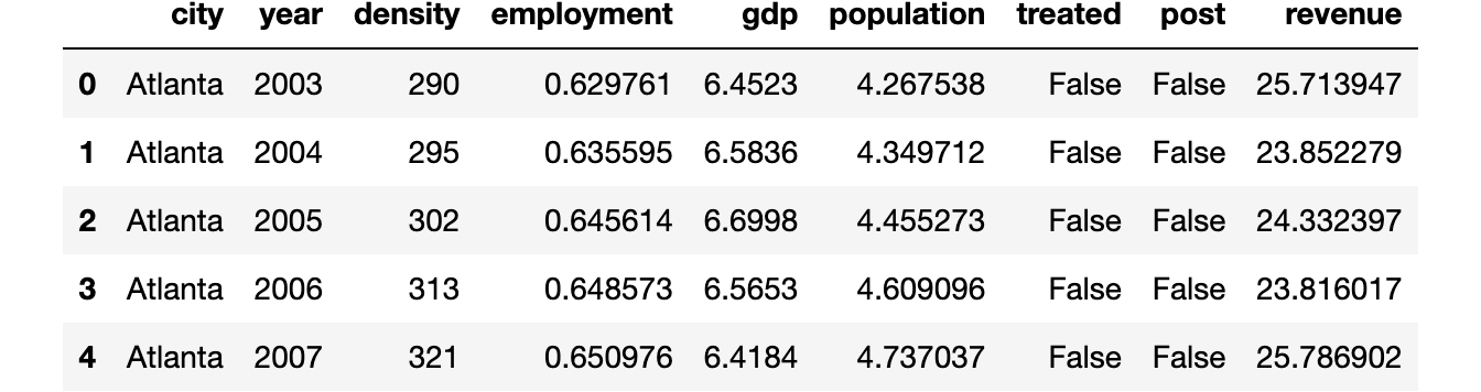
We’ve data on the most important 46 U.S. cities for the interval 2002–2019. The panel is balanced, which implies that we observe all cities all the time durations. Self-driving automobiles had been launched in 2013.
Is the handled unit, Miami, corresponding to the remainder of the pattern? Let’s use the create_table_one operate from Uber’s causalml package deal to supply a covariate stability desk, containing the typical worth of our observable traits, throughout remedy and management teams. Because the title suggests, this could all the time be the primary desk you current in causal inference evaluation.
from causalml.match import create_table_onecreate_table_one(df, 'handled', ['density', 'employment', 'gdp', 'population', 'revenue'])

As anticipated, the teams are not balanced: Miami is extra densely populated, poorer, bigger, and has a decrease employment charge than the opposite cities within the US in our pattern.
We’re fascinated by understanding the affect of the introduction of self-driving automobiles on income.
One preliminary thought may very well be to investigate the information as we’d in an A/B check, evaluating the management and remedy group. We are able to estimate the remedy impact as a distinction in means in income between the remedy and management teams, after the introduction of self-driving automobiles.
smf.ols('income ~ handled', knowledge=df[df['post']==True]).match().abstract().tables[1]

The impact of self-driving automobiles appears to be destructive however not important.
The primary downside right here is that remedy was not randomly assigned. We’ve a single handled unit, Miami, and it’s hardly corresponding to different cities.
One various process is to match income earlier than and after the remedy, throughout the metropolis of Miami.
smf.ols('income ~ publish', knowledge=df[df['city']==treated_city]).match().abstract().tables[1]

The impact of self-driving automobiles appears to be constructive and statistically important.
Nevertheless, the downside with this process is that there may need been many different issues taking place after 2013. It’s fairly a stretch to attribute all variations to self-driving automobiles.
We are able to higher perceive this concern if we plot the time development of income over cities. First, we have to reshape the information right into a huge format, with one column per metropolis and one row per yr.
df = df.pivot(index='yr', columns='metropolis', values='income').reset_index()
Now, let’s plot the income over time for Miami and for the opposite cities.
cities = [c for c in df.columns if c!='year']
df['Other Cities'] = df[[c for c in cities if c != treated_city]].imply(axis=1)
Since we’re speaking about Miami, let’s use an applicable shade palette.
sns.set_palette(sns.color_palette(['#f14db3', '#0dc3e2', '#443a84']))plot_lines(df, treated_city, 'Different Cities', treatment_year)

As we will see, income appears to be growing after the remedy in Miami. Nevertheless it’s a really unstable time sequence. And income was growing additionally in the remainder of the nation. It’s very arduous from this plot to attribute the change to self-driving automobiles.
Can we do higher?
The reply is sure! Artificial management permits us to do causal inference when we have now as few as one handled unit and many management items and we observe them over time. The concept is straightforward: mix untreated items in order that they mimic the habits of the handled unit as intently as attainable, with out the remedy. Then use this “artificial unit” as a management. The strategy was first launched by Abadie, Diamond, and Hainmueller (2010) and has been known as “a very powerful innovation within the coverage analysis literature in the previous few years”. Furthermore, it’s broadly used within the trade due to its simplicity and interpretability.
Setting
We assume that for a panel of i.i.d. topics i = 1, …, n over time t=1, …,T we noticed a set of variables (Xᵢₜ,Dᵢ,Yᵢₜ) that features
- a remedy project Dᵢ∈{0,1} (
handled) - a response Yᵢₜ∈ℝ(
income) - a characteristic vector Xᵢₜ∈ℝⁿ (
inhabitants,density,employmentandGDP)
Furthermore, one unit (Miami in our case) is handled at time t* (2013 in our case). We distinguish time durations earlier than remedy and time durations after remedy.
Crucially, remedy D just isn’t randomly assigned, due to this fact a distinction in means between the handled unit(s) and the management group just isn’t an unbiased estimator of the typical remedy impact.
The Downside
The issue is that, as regular, we don’t observe the counterfactual end result for handled items, i.e. we have no idea what would have occurred to them if that they had not been handled. This is called the basic downside of causal inference.
The only strategy can be simply to match pre- and post-treatment durations. That is known as the occasion examine strategy.
Nevertheless, we will do higher than this. In reality, regardless that remedy was not randomly assigned, we nonetheless have entry to some items that weren’t handled.
For the end result variable, we observe the next values

The place Y⁽ᵈ⁾ₐ,ₜ is the end result at time t, given remedy project a and remedy standing d. We mainly have a lacking knowledge downside since we don’t observe Y⁽⁰⁾ₜ,ₚₒₛₜ: what would have occurred to handled items (a=t) with out remedy (d=0).
The Answer
Following Doudchenko and Inbens (2018), we will formulate an estimate of the counterfactual end result for the handled unit as a linear mixture of the noticed outcomes for the management items.

the place
- the fixed α permits for various averages between the 2 teams
- the weights βᵢ are allowed to differ throughout management items i (in any other case, it might be a difference-in-differences)
How ought to we select which weights to make use of? We wish our artificial management to approximate the end result as intently as attainable, earlier than the remedy. The primary strategy may very well be to outline the weights as

I.e. the weights are such that they reduce the space between observable traits of management items Xc and the handled unit Xₜ earlier than the remedy.
You would possibly discover a really shut similarity to linear regression. Certainly, we’re doing one thing very related.
In linear regression, we normally have many items (observations), few exogenous options, and one endogenous characteristic and we attempt to categorical the endogenous characteristic as a linear mixture of the endogenous options, for every unit.

With artificial management, we as an alternative have many time durations (options), few management items and a single handled unit and we attempt to categorical the handled unit as a linear mixture of the management items, for every time interval.
To carry out the identical operation, we basically must transpose the information.

After the swap, we compute the artificial management weights, precisely as we’d compute regression coefficients. Nevertheless, now one commentary is a time interval and one characteristic is a unit.

Discover that this swap is not harmless. In linear regression we assume that the connection between the exogenous options and the endogenous characteristic is similar throughout items, as an alternative in artificial management we assume that the connection between the handled items and the management unit is similar over time.
Again to self-driving automobiles
Let’s return to the information now! First, we write a synth_predict operate that takes as enter a mannequin that’s skilled on management cities and tries to foretell the end result of the handled metropolis, Miami, earlier than the introduction of self-driving automobiles.
Let’s estimate the mannequin by way of linear regression.
from sklearn.linear_model import LinearRegressioncoef = synth_predict(df, LinearRegression(), treated_city, treatment_year).coef_
How effectively did we match pre-self-driving automobiles income in Miami? What’s the implied impact of self-driving automobiles?
We are able to visually reply each questions by plotting the precise income in Miami in opposition to the anticipated one.
plot_lines(df, treated_city, f'Artificial {treated_city}', treatment_year)

It seems to be like self-driving automobiles had a wise constructive impact on income in Miami: the anticipated development is decrease than the precise knowledge and diverges proper after the introduction of self-driving automobiles.
However, we’re clearly overfitting: the pre-treatment predicted income line is completely overlapping with the precise knowledge. Given the excessive variability of income in Miami, that is suspicious, to say the least.
One other downside considerations the weights. Let’s plot them.
df_states = pd.DataFrame({'metropolis': [c for c in cities if c!=treated_city], 'ols_coef': coef})
plt.determine(figsize=(10, 9))
sns.barplot(knowledge=df_states, x='ols_coef', y='metropolis');

We’ve many destructive weights, which don’t make a lot sense from a causal inference perspective. I can perceive that Miami may be expressed as a mixture of 0.2 St. Louis, 0.15 Oklahoma, and 0.15 Hartford. However what does it imply that Miami is -0.15 Milwaukee?
Since we wish to interpret our artificial management as a weighted common of untreated states, all weights must be constructive and they need to sum to at least one.
To deal with each considerations (weighting and overfitting), we have to impose some restrictions on the weights.
Restricted Weights
To resolve the issues of overweighting and destructive weights, Abadie, Diamond, and Hainmueller (2010) suggest the next weights:
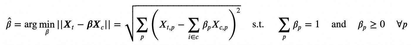
This implies, a set of weights β such that
- weighted observable traits of the management group Xc, match the observable traits of the remedy group Xₜ, earlier than the remedy
- they sum to 1
- and will not be destructive.
With this strategy, we get an interpretable counterfactual as a weighted common of untreated items.
Let’s write now our personal goal operate. I create a brand new class SyntheticControl() which has each a loss operate, as described above, a technique to match it and predict the values for the handled unit.
We are able to now repeat the identical process as earlier than however utilizing the SyntheticControl methodology as an alternative of the straightforward, unconstrained LinearRegression.
df_states['coef_synth'] = synth_predict(df, SyntheticControl(), treated_city, treatment_year).coef_
plot_lines(df, treated_city, f'Artificial {treated_city}', treatment_year)

As we will see, now we’re not overfitting anymore. The precise and predicted income pre-treatment are shut however not similar. The reason being that the non-negativity constraint is constraining most coefficients to be zero (as Lasso does).
It seems to be just like the impact is once more destructive. Nevertheless, let’s plot the distinction between the 2 traces to raised visualize the magnitude.
plot_difference(df, treated_city, treatment_year)

The distinction is clearly constructive and barely growing over time.
We are able to additionally visualize the weights to interpret the estimated counterfactual (what would have occurred in Miami, with out self-driving automobiles).
plt.determine(figsize=(10, 9))
sns.barplot(knowledge=df_states, x='coef_synth', y='metropolis');

As we will see, now we’re expressing income in Miami as a linear mixture of simply a few cities: Tampa, St. Louis and, to a decrease extent, Las Vegas. This makes the entire process very clear.
What about inference? Is the estimate considerably completely different from zero? Or, extra virtually, “how uncommon is that this estimate beneath the null speculation of no coverage impact?”.
We’re going to carry out a randomization/permutation check so as to reply this query. The thought is that if the coverage has no impact, the impact we observe for Miami shouldn’t be considerably completely different from the impact we observe for another metropolis.
Subsequently, we’re going to replicate the process above, however for all different cities and examine them with the estimate for Miami.
fig, ax = plt.subplots()
for metropolis in cities:
synth_predict(df, SyntheticControl(), metropolis, treatment_year)
plot_difference(df, metropolis, treatment_year, vline=False, alpha=0.2, shade='C1', lw=3)
plot_difference(df, treated_city, treatment_year)

From the graph, we discover two issues. First, the impact for Miami is sort of excessive and due to this fact probably to not be pushed by random noise.
Second, we additionally discover that there are a few cities for which we can’t match the pre-trend very effectively. Specifically, there’s a line that’s sensibly decrease than all others. That is anticipated since, for every metropolis, we’re constructing the counterfactual development as a convex mixture of all different cities. Cities which are fairly excessive by way of income are very helpful to construct the counterfactuals of different cities, but it surely’s arduous to construct a counterfactual for them.
To not bias the evaluation, let’s exclude states for which we can’t construct a “adequate” counterfactual, by way of pre-treatment MSE.

As a rule of thumb, Abadie, Diamond, and Hainmueller (2010) recommend excluding items for which the prediction MSE is bigger than twice the MSE of the handled unit.
# Reference mse
mse_treated = synth_predict(df, SyntheticControl(), treated_city, treatment_year).mse# Different mse
fig, ax = plt.subplots()
for metropolis in cities:
mse = synth_predict(df, SyntheticControl(), metropolis, treatment_year).mse
if mse < 2 * mse_treated:
plot_difference(df, metropolis, treatment_year, vline=False, alpha=0.2, shade='C1', lw=3)
plot_difference(df, treated_city, treatment_year)

After excluding excessive observations, it seems to be just like the impact for Miami could be very uncommon.
One statistic that Abadie, Diamond, and Hainmueller (2010) recommend to carry out a randomization check is the ratio between pre-treatment MSE and post-treatment MSE.

We are able to compute a p-value because the variety of observations with a better ratio.
p-value: 0.04348
It appears that evidently solely 4.3% of the cities had a bigger MSE ratio than Miami, implying a p-value of 0.043. We are able to visualize the distribution of the statistic beneath permutation with a histogram.
fig, ax = plt.subplots()
_, bins, _ = plt.hist(lambdas.values(), bins=20, shade="C1");
plt.hist([lambdas[treated_city]], bins=bins)
plt.title('Ratio of $MSE_{publish}$ and $MSE_{pre}$ throughout cities');
ax.add_artist(AnnotationBbox(OffsetImage(plt.imread('fig/miami.png'), zoom=0.25), (2.7, 1.7), frameon=False));

Certainly, the statistic for Miami is sort of excessive, indicating that it’s unlikely that the noticed impact is because of noise.
On this article, we have now explored a very talked-about methodology for causal inference when we have now few handled items, however many time durations. This setting emerges usually in trade settings when the remedy must be assigned on the combination stage and randomization won’t be attainable. The important thing thought of artificial management is to combinate management items into one artificial management unit to make use of as counterfactual to estimate the causal impact of the remedy.
One of many primary benefits of artificial management is that, so long as we use constructive weights which are constrained to sum to at least one, the tactic avoids extrapolation: we are going to by no means exit of the help of the information. Furthermore, artificial management research may be “pre-registered”: you may specify the weights earlier than the examine to keep away from p-hacking and cherry-picking. One more reason why this methodology is so standard within the trade is that weights make the counterfactual evaluation specific: one can take a look at the weights and perceive which comparability we’re making.
This methodology is comparatively younger and lots of extensions are showing yearly. Some notable ones are the generalized artificial management by Xu (2017), the artificial difference-in-differences by Doudchenko and Imbens (2017), and the penalized artificial management of Abadie e L’Hour (2020), and the matrix completion strategies of Athey et al. (2021). Final however not least, if you wish to have the tactic defined by one in all its inventors, there may be this nice lecture by Alberto Abadie on the NBER Summer time Institute freely obtainable on Youtube.
References
[1] A. Abadie, A. Diamond, J. Hainmueller, Artificial Management Strategies for Comparative Case Research: Estimating the Impact of California’s Tobacco Management Program (2010), Journal of the American Statistical Affiliation.
[2] A. Abadie, Utilizing Artificial Controls: Feasibility, Knowledge Necessities, and Methodological Points (2021), Journal of Financial Views.
[3] N. Doudchenko, G. Imbens, Balancing, Regression, Distinction-In-Variations and Artificial Management Strategies: A Synthesis (2017), working paper.
[4] Y. Xu, Generalized Artificial Management Methodology: Causal Inference with Interactive Fastened Results Fashions (2018), Political Evaluation.
[5] A. Abadie, J. L’Hour, A Penalized Artificial Management Estimator for Disaggregated Knowledge (2020), Journal of the American Statistical Affiliation.
[6] S. Athey, M. Bayati, N. Doudchenko, G. Imbens, Okay. Khosravi, Matrix Completion Strategies for Causal Panel Knowledge Fashions (2021), Journal of the American Statistical Affiliation.
Associated Articles
Knowledge
Code
You could find the unique Jupyter Pocket book right here:
Thanks for studying!
I actually respect it!  In case you preferred the publish and wish to see extra, think about following me. I publish as soon as every week on subjects associated to causal inference and knowledge evaluation. I attempt to hold my posts easy however exact, all the time offering code, examples, and simulations.
Additionally, a small disclaimer: I write to study so errors are the norm, regardless that I attempt my finest. Please, if you spot them, let me know. I additionally respect solutions on new subjects!
