
Statistics in R Sequence

Introduction
R is a really highly effective programming language for statistical analyses. There are a number of programming platforms for statistical evaluation however R has gained actual attraction amongst information scientists and information analysts due to its inherent functionality to carry out statistical duties higher than others and ship the visualizations extra aesthetically. On this article, I’m going to display the interpretation of very fundamental statistical instructions executed in R. Anybody can carry out the duties on a number of different platforms however we have to perceive the true thought behind its execution as a result of these statistical ideas are timeless. The software program, this system, the versions-everything can get up to date however the ideas behind this statistical evaluation won’t change.
Knowledge
For demonstration, I’ll use the Basic Social Survey (GSS) information collected in 2016. The information had been downloaded from the Affiliation of Faith Knowledge Archives and had been collected by Tom W. Smith. This information set has responses collected from practically 3,000 respondents and it has information associated to a number of socio-economic options. For instance, it has information associated to marital standing, schooling background, working hours, employment standing, and lots of extra. Let’s dive into this dataset I perceive it a bit extra.
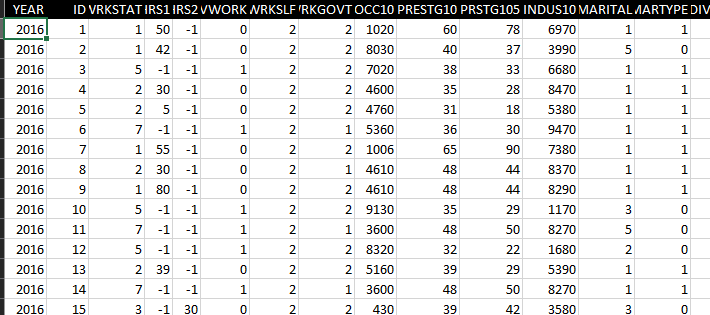
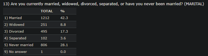
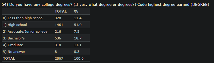
The outline of MARITAL and DEGREE encoded values are proven beneath since we’ll use these options in subsequent analyses.
This information set includes a number of options both quantitative or categorical. The explicit information are additionally encoded ordinally. For instance, the schooling background has six totally different classes and every of those classes is assigned a quantity ranging from 0. The gender can be categorical and solely two values are assigned for this function: “1” for males and “2” for females. There are additionally a number of quantitative information instance age. To grasp extra concerning the assigned numbers, the reader must go to the given hyperlink and discover out which quantity is related to which categorical worth. We are going to use this information and execute the next instructions on each categorical and quantitative information and interpret the outputs.
The libraries are additionally proven right here. I’ll use Rstudio. The purpose is to grasp the outputs from these instructions, not emphasize the syntax.
Group_by
The group_by is likely one of the most simple and extensively used instructions for any type of evaluation. It teams the info based mostly on the given function variable. As soon as this group_by command is executed and saved in a variable, we are able to summarize that variable and show the specified statistics.
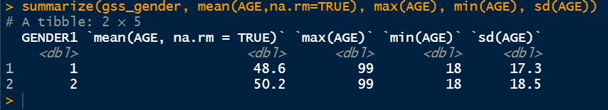
The above command exhibits the imply, the utmost, the minimal, and the usual deviation of age grouped by totally different genders that are very important statistics for any dataset.
Group_by with descr
Different necessary statistics could be decided by combining descr command with group_by.
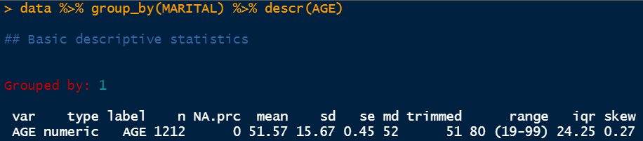
The above snap exhibits that the info is grouped by group 1 and the variable it’s describing is AGE. The kind of the variable is numeric and it has a complete of 1212 information factors the quantity of null values is 0. It has a imply of 51.57 and a regular deviation of 15.67. Then we now have a regular error which is denoted by se right here. The usual error is the usual deviation divided by the entire variety of information factors. On this case, it’s 15.67/1212. Subsequent, we now have the median worth which is 52. It says that the median age of the individuals belonging to group 1 is 52. Group 1 is the group for married individuals. Then we now have the trimmed vary which is displaying right here 51–80. It primarily eliminates a share of the decrease and the higher information factors however the true vary is displaying subsequent which is nineteen–99. The IQR worth is decided as 24.25 which is the distinction between the third quartile and the primary quartile (Q3-Q1). The IQR worth could be very helpful to find out the higher restrict and decrease restrict for field plots to eradicate the outliers. Lastly, we now have the skew worth which is 0.27. This worth signifies that the distribution is pretty regular. Any worth above 1 is just about right-skewed and any worth beneath -1 is taken into account left-skewed.
Statistics by chosen options
We are able to additionally decide varied statistics of various parameters utilizing totally different libraries. A kind of executions is proven beneath.
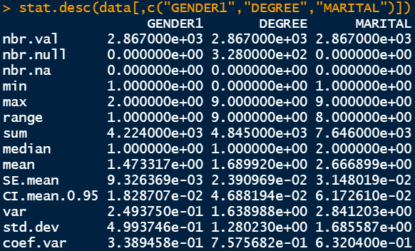
The output exhibits the entire variety of information factors within the first row and the entire variety of null values within the second and the third row. Following that, we now have the minimal and the utmost worth in addition to the vary worth. The sum, the median, the typical, and the usual error are additionally proven in subsequent rows. We even have the worth of 95% confidence interval imply information. Then, we even have the variance and the usual deviation values in addition to the coefficient of variance. Variance is the sq. of normal deviation and coefficient of variance is the usual deviation divided by the imply. Normal deviation is the first variable of curiosity to find out the unfold of the specified parameter. Nevertheless, coefficient of variance is one other option to measure the unfold by way of the imply.
Desk command
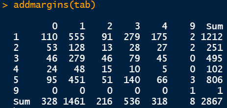
Desk is a really highly effective command to visualise the info cut up into two totally different teams. For instance, within the following determine, the info is cut up into two teams: the primary group is the marital standing and the second group is the diploma standing.
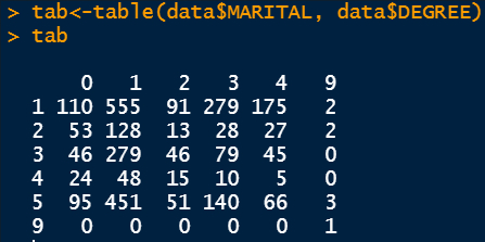
Because the categorical variables are encoded, we have to refer again to the outline of the dataset to grasp the underlying relation. For instance 0 within the row refers to individuals having an schooling background lower than highschool and 1 within the column refers to people who find themselves married. Due to this fact, 110 individuals have an schooling background lower than highschool and are married. There are totally different numbers because the schooling background adjustments.
Different miscellaneous instructions
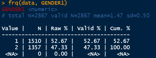
The frequency command denoted by frq determines necessary statistics of the chosen function. It exhibits the share values moreover in addition to the cumulative percentages.
The abstract command exhibits the Chi-Sq. check output if a number of components are chosen. We are able to feed the beforehand decided tab variable.
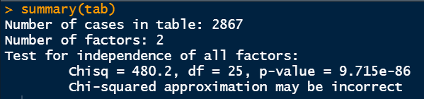
I want to make clear these numbers from Chi-Sq. check. Initially, the tab variable holds the desk information from marital standing and schooling background standing. What the Chi-Sq. check is doing is, it’s checking the independence of 1 variable from one other variable. Right here, the Chi-Sq. check is checking if there’s any dependency of the schooling background represented by DEGREE is by some means associated to the marital standing represented by MARITAL.
It does the calculation of p-value from the speculation check. The null speculation right here states that the variables of curiosity (MARITAL and DEGREE) usually are not depending on one another. The choice speculation says that the variables are associated and there could also be some type of correlation. On this case, the p-value could be very small. The same old significance degree is 5%. Because the p-value is lower than 0.05, we are able to reject the null speculation and conclude that the schooling background is said to marital standing.
The addmargins command gives the row and column summations.
Crosstable
Crosstable command is one other very highly effective command to visualise the desk outputs and get extra statistics.
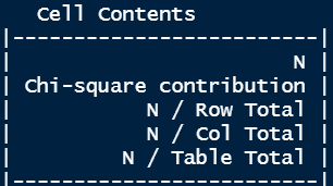
Other than the quantity (N), it additionally gives the Chi-Sq. contribution, the share in the direction of the entire of every row in addition to every column, and the share of the entire quantity.
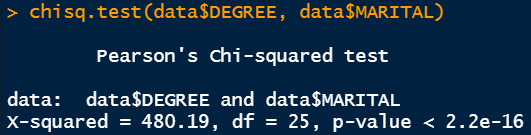
We are able to additionally decide the chi-square worth and the corresponding p-value as proven beneath. It additionally gives the identical statistics. The Chi-Sq. worth is 480.19 and the diploma of freedom is 25. Within the output of the crosstable command, you possibly can see the contribution of every phase in the direction of this complete Chi-Sq. worth of 480.19. The diploma of freedom worth is calculated by multiplying (variety of rows -1) and (variety of columns -1).
Conclusion
Now we have lined probably the most fundamental interpretation of a number of important R instructions required for statistical evaluation. These are required for each categorical and quantitative information evaluation though the following steps i.e. regression could be proceeded in another way.
Thanks for studying.
