
Demonstrating how background works in Neural Networks, utilizing an instance
Neural Networks study by means of iterative tuning of parameters (weights and biases) throughout the coaching stage. At first, parameters are initialized by randomly generated weights, and the biases are set to zero. That is adopted by a ahead go of the info by means of the community to get mannequin output. Lastly, back-propagation is performed. The mannequin coaching course of usually entails a number of iterations of a ahead go, back-propagation, and parameters replace.
This text will concentrate on how back-propagation updates the parameters after a ahead go (we already lined ahead propagation within the earlier article). We’ll work on a easy but detailed instance of back-propagation. Earlier than we proceed, let’s see the info and the structure we are going to use on this put up.
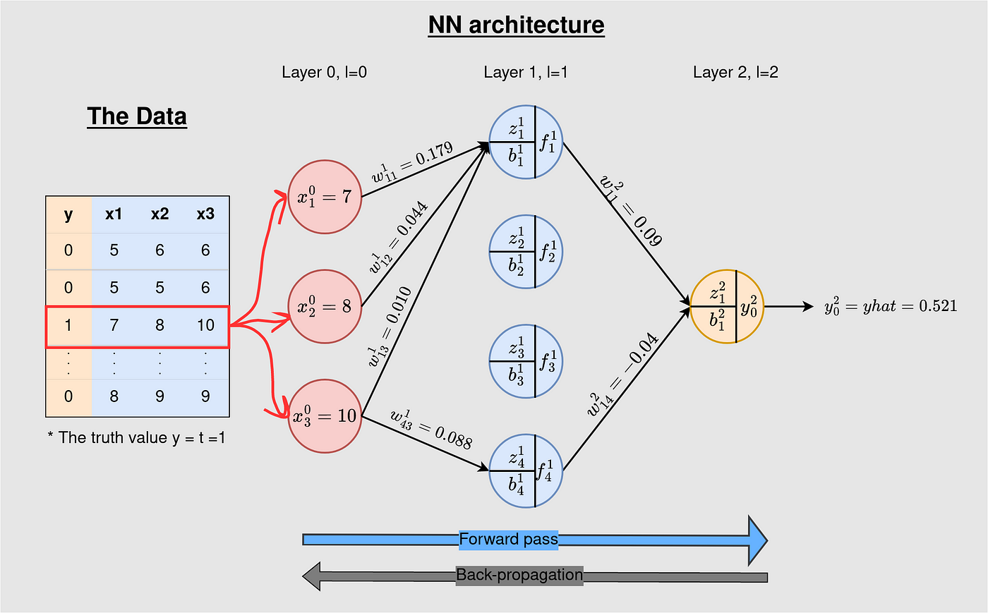
The dataset used on this article incorporates three options, and the goal class has solely two values — 1 for go and 0 for fail. The target is to categorise a knowledge level into both of the 2 classes — a case of binary classification. To make the instance simply comprehensible, we are going to use just one coaching instance on this put up.
Perceive: A ahead go permits the knowledge to move in a single route — from enter to the output layer, whereas the back-propagation does the reverse — permitting knowledge to move from output backward whereas updating the parameters (weights and biases).
Definition: Again-propagation is a technique for supervised studying utilized by NN to replace parameters to make the community’s predictions extra correct. The parameter optimization course of is achieved utilizing an optimization algorithm referred to as gradient descent (this idea might be very clear as you learn alongside).
A ahead go yields a prediction (yhat) of the goal (y) at a loss which is captured by a price perform (E) outlined as:
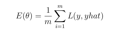
the place m is the variety of coaching examples, and L is the error/loss incurred when the mannequin predicts yhat as a substitute of precise worth y. The target is to reduce the fee E. That is achieved by differentiating E with respect to (wrt) parameters (weights and parameters) and adjusting the parameters in the other way of the gradient (that’s the reason the optimization algorithm is known as gradient descent).
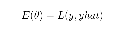
On this put up, we think about back-propagation on 1 coaching instance (m=1). With this consideration, E, reduces to
The loss perform, L, is outlined primarily based on the duty at hand. For classification issues, Cross-entropy (also referred to as log loss) and hinge loss are appropriate loss capabilities, whereas, Imply Squared Error (MSE) and Imply Absolute Error (MAE) are acceptable loss capabilities for regression duties.
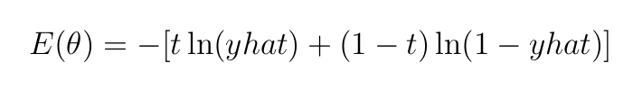
Binary cross-entropy loss is a perform appropriate for our binary classification process — the info has two courses, 0 or 1. A binary cross-entropy loss perform will be utilized to our forward-pass instance in Determine 1, as proven under
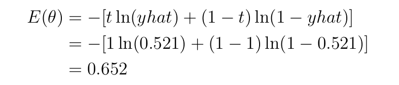
t=1 is the reality label, yhat=0.521 is the output of the mannequin and ln is the pure log— log to base 2.
You’ll be able to learn extra concerning the cross entropy loss perform on the hyperlink under.
Since we now perceive the NN structure and the fee perform we are going to use, we are able to proceed on to cowl the steps for backward propagation.
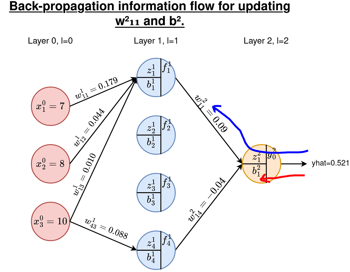
The desk under reveals the info on all of the layers of the 3–4–1 NN. On the 3-neuron enter, the values proven are from the info we offer to the mannequin for coaching. The second/hidden layer incorporates the weights (w) and biases (b) we want to replace and the output (f) at every of the 4 neurons throughout the ahead go. The output incorporates the parameters (w and b) and the output of the mannequin (yhat) — this worth is definitely the mannequin prediction at every iteration of mannequin coaching. After a single forward-pass, yhat=0.521.

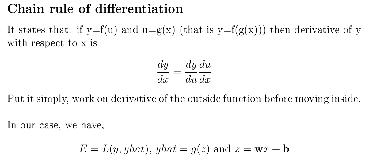
Essential: Recall from the earlier part: E(θ)=L(y, yhat) the place θ is our parameters — weights and biases. That’s to say, E is a perform of y and yhat and yhat=g(wx+b), => yhat is a perform of w and b. x is a variable of information and g is the activation perform. Successfully, E is a perform w and b and, due to this fact will be differentiated with respect to those parameters.
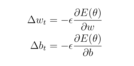
The parameters at every layer are up to date with the next equations

the place t is the training step, ϵ is the training charge — a hyper-parameter set by the person. It determines the speed at which the weights and biases are up to date. We’ll use ϵ=0.5 (arbitrary selection).
From Equations 4, the replace quantities turns into
As stated earlier, since we’re coping with binary classification, we are going to use the binary cross-entropy loss perform outlined as:
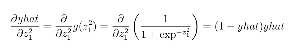
We’ll use Sigmoid activation throughout all layers
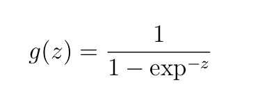
the place z=wx+b is the weighted enter into the neuron plus bias.
Not like the ahead go, again prop works backward from the output layer to layer 1. We have to compute derivatives/gradients with respect to parameters for all layers. To do this, we’ve got to grasp the chain rule of differentiation.
Let’s work on updating w²₁₁ and b²₁ as examples. We’ll comply with the routes proven under.
B1. Calculating Derivatives for the Weights
By chain rule of differentiation, we’ve got
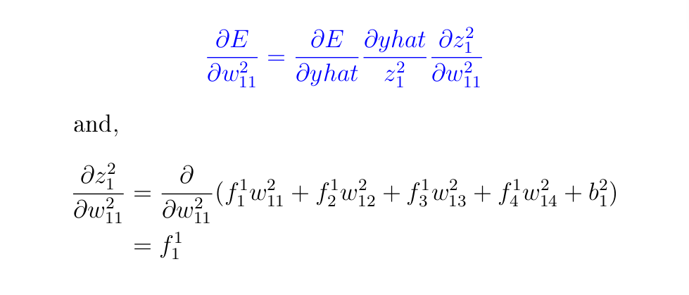
Keep in mind: when evaluating the above derivatives with respect to w²₁₁, all the opposite parameters are handled as constants, that’s, w²₁₂, w²₁₃, w²₁₄, and b²₁. The by-product of a continuing is 0 that’s the reason some values have been eradicated within the above by-product.
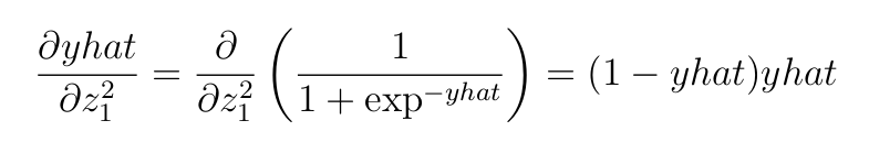
Subsequent is the by-product of Sigmoid perform (please affirm this by-product)
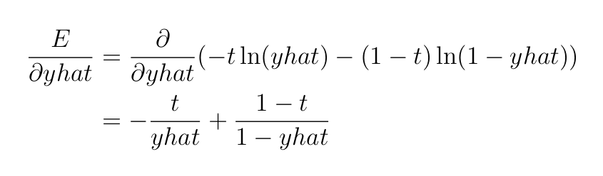
Subsequent, the by-product of cross-entropy loss perform (additionally verify this)
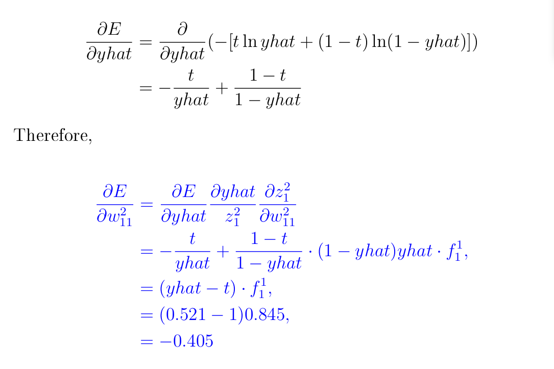
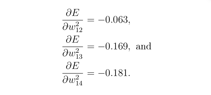
The derivatives with the respect to the opposite three weights on the output layer are as follows (you’ll be able to affirm this)
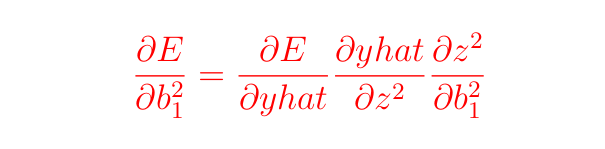
B2. Computing Derivatives for the bias
We have to compute
From the earlier sections, we’ve got already computed ∂E and ∂yhat, what stays is
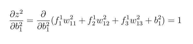
We used the identical arguments as earlier than, that every one different variables besides b²₁ are handled as constants due to this fact on when differentiated they cut back 0.

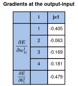
To date, we’ve got computed the gradients with respect to all of the parameters on the output-input layers.
At this level we’re able to replace all of the weights and biases on the output-input layers.
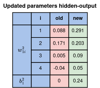
B3. Updating Parameters on the Output-Enter Layers
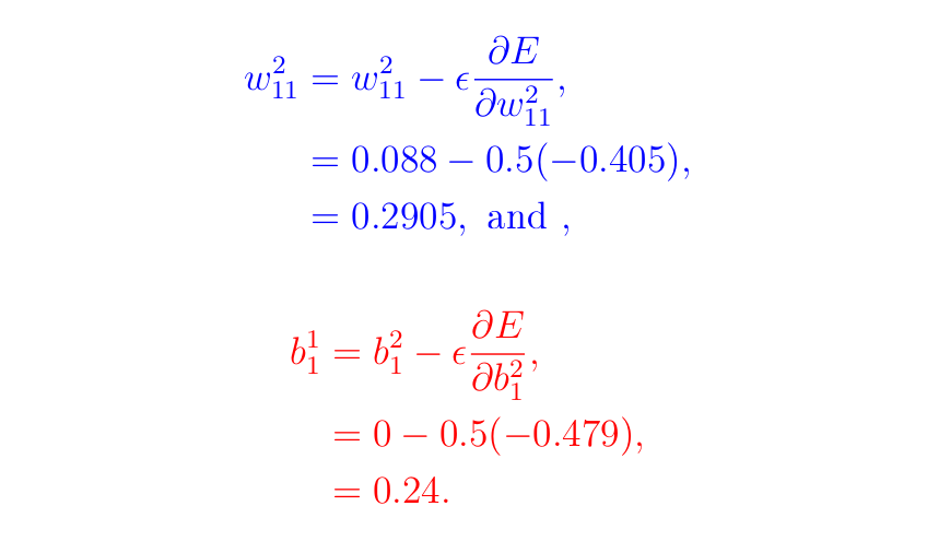
Please compute the remaining in the identical manner and ensure them within the desk under
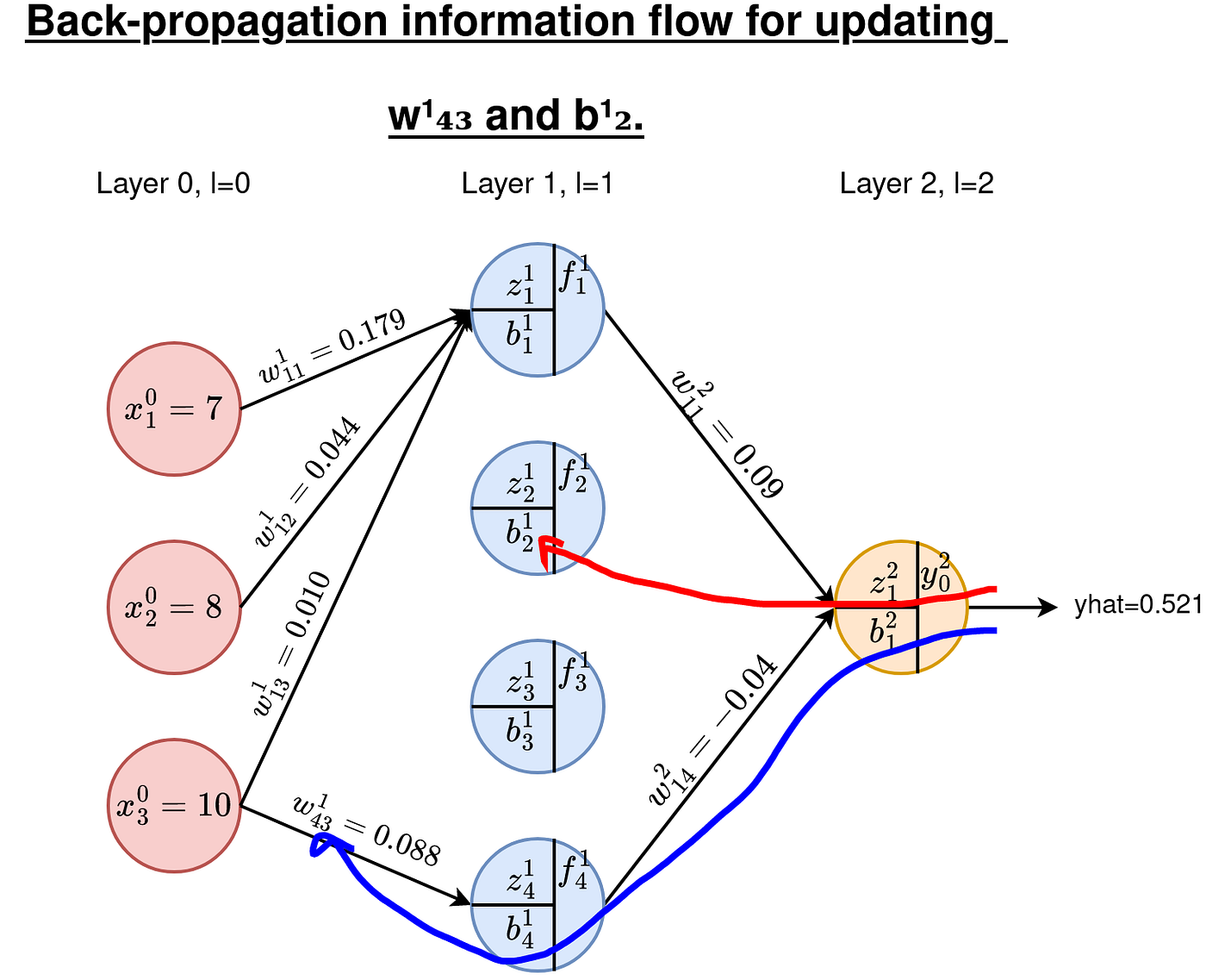
As earlier than, we’d like derivatives of E with respect to all of the weights and biases at these layers. We now have a complete of 4x3=12 weights to replace and 4 biases. As instance, lets work on w¹₄₃ and b¹₂. See the routes within the Determine under.
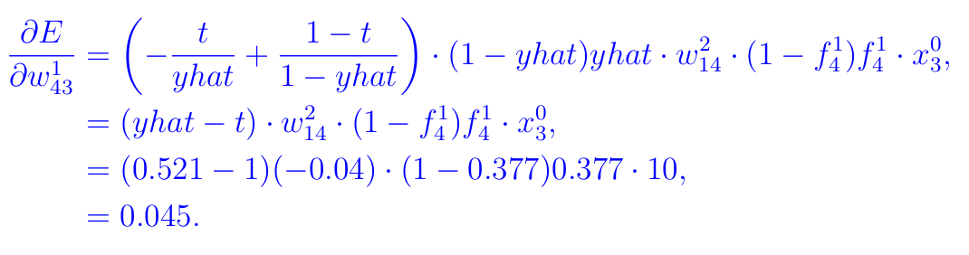
C1. Gradients of weights
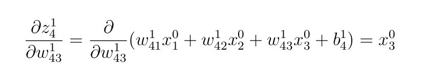
For weights, we have to compute the by-product (comply with the route in Determine 6 if the next equation is intimidating)

As we undergo every of the above derivatives, be aware the next essential factors:
- On the mannequin output (when discovering by-product of
Ewith respect to theyhat), we are literally differentiating the loss perform. - On the layer outputs (
f) (the place we differentiate wrtz), we discover the activation perform’s by-product. - Within the above two instances, differentiating with respect to weights or biases of a given neuron yields the identical outcomes.
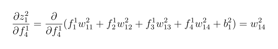
- The weighted inputs (
z) are differentiated with respect to parameters (worb) that we want to replace. On this case, all parameters are held fixed besides the parameter of curiosity.
Doing the identical course of as in Part B, we get:
- weighted inputs for layer
1
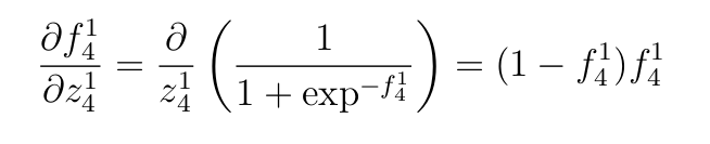
- by-product of Sigmoid activation perform utilized to the primary layer
- Weighted inputs to the output layer.
f-values are the outputs of the hidden layer.
- Activation perform utilized to the output of the final layer.
- Spinoff of binary cross-entropy loss perform wrt to
yhat.
Then, we are able to put collectively all these as
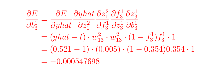
C2. Gradients of bias
Utilizing the identical ideas as earlier than, verify that, for b¹₂, we’ve got
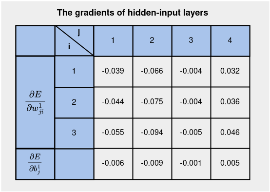
All gradient values for the hidden-input are tabulated under
At this level, we’re able to compute the up to date parameters on the hidden-input.
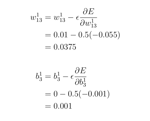
C3. Updating Parameters on the Hidden-Enter
Lets return to the replace equations and work on updating w¹₁₃ and b¹₃
So, what number of parameters do we’ve got to replace?
We now have 4x3=12 weights and 4x1=4 biases on the hidden-input layers, 4x1=4 weights, and 1 bias on the output-hidden layers. That could be a whole of 21 parameters. They’re referred to as trainable parameters.
All of the up to date parameters for hidden-input layers are proven under
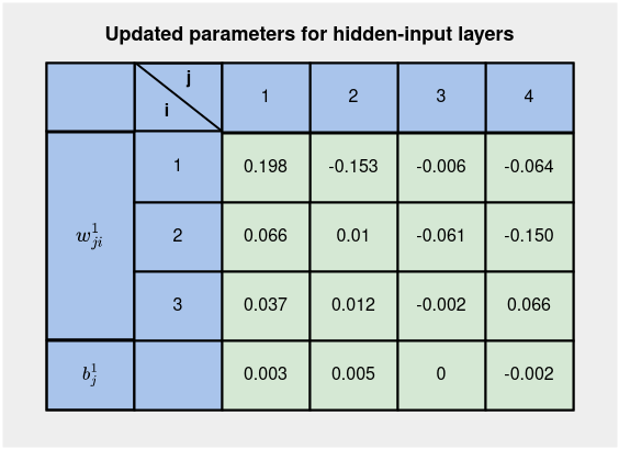
We now have the up to date parameters for all of the layers in Determine 8 and Determine 5 utilizing back-propagation of error. Working a ahead go with these up to date parameters yields a mannequin prediction, yhat of 0.648, up from 0.521. Which means that a mannequin is studying — shifting near the true worth of 1 after two iterations of coaching. Different iterations yield 0.758, 0.836, 0.881, 0.908, 0.925, … (Within the subsequent article, we are going to implement back-propagation and ahead go for a lot of coaching examples and iterations, and you’ll get to see this).
- Epoch — One epoch is when all the dataset is handed by means of the community as soon as. This includes of 1 occasion of a ahead go and back-propagation.
- Tub measurement is the variety of coaching examples handed by means of the community concurrently. In our case, we’ve got one coaching instance. In instances the place we’ve got a big dataset, the info will be handed by means of the community in batches.
- The variety of iterations — One iteration equals one go utilizing coaching examples set as batch measurement. One go is a ahead go and a back-propagation.
Instance:
If we’ve got 2000 coaching examples and set batch measurement of 20, then it takes 100 iterations to finish 1 epoch.
On this article, we’ve got mentioned back-propagation by engaged on an instance. We now have seen how chain rule of differentiation is used to get the gradients of various equations — the loss perform, activation perform, weighting equations and layer output equations. We now have additionally mentioned on how by-product with respect to the loss perform can be utilized to replace parameters at every layer. Within the subsequent article, we are going to implement the ideas learnt right here in Python. We’ll conduct full coaching of a neural community with a big dataset (not only one coaching instance) and conduct many iterations of ahead and again go.
