A way for calculating delay possibilities on a given connection utilizing Python
1. Introduction
Delays have at all times been a part of our day by day lives, primarily as a result of most of us have used public transportation from a younger age to maneuver from one level to a different.
Let’s now ask ourselves a query. Given a connection, how seemingly is a delay? Wouldn’t it’s useful to have the ability to choose the route with the least delay so you may arrive on the vacation spot on time?
Immediately I wish to discuss to you about likelihood distributions in public transport delays. What I imply by that’s understanding the distribution of delays and tips on how to implement this probabilistic downside utilizing Python simply.
Each day life software
For instance of how delay possibilities may very well be used, here’s a screenshot from a prepare timetable app I’ve constructed for a undertaking at my college [2].
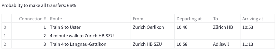
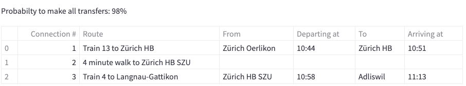
As we will see from the tables, the app permits us to decide on the route that finest meets our wants: we might take the shorter method that can allow us to depart 2 minutes later however solely has a 66% probability of arriving on time, or we might take the longer route, and have a 98% probability of arriving on time.
This easy instance demonstrates the potential and significance of likelihood distributions in our day by day lives.
2. Dataset
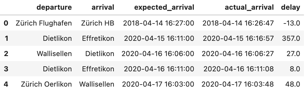
Because of a college undertaking, I’ve come throughout a dataset from the Swiss public transport system. As you may see beneath, this dataset accommodates historic information relating to station arrival instances.

Along with station info and metadata, it consists of columns for expected_arrival time and actual_arrival time. Utilizing these, we will get the delay for a given day at a given time.
For the sake of simplicity, let’s take into account solely the connection departing from “Zürich Flughafen” and arriving at “Zürich HB”.
delay_connection = df[(df["departure"] == "Zürich Flughafen") & (df["arrival"]=="Zürich HB")]
3. Distributions
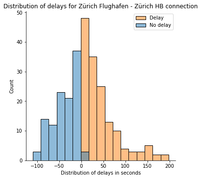
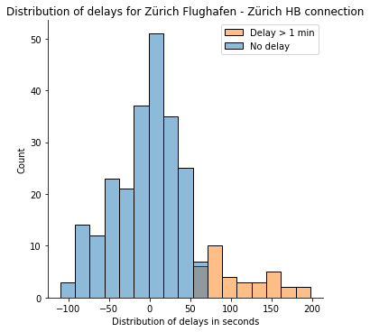
Now we will present the distribution of delays for this connection.

As we will see from the distribution, evidently it tends in the direction of a standard / log-normal distribution. Many research have been carried out to investigate the distribution of delays, and for extra element, I counsel taking a look at [1]. On this publish, we are going to assume that the distribution is regular.
4. Calculating distribution and possibilities
Now, we have to mannequin our distribution to find out the likelihood {that a} delay will happen. We begin by getting the imply and commonplace deviation of delays on a given connection.
mean_delay = delay_connection.delay.imply()
std_delay = delay_connection.delay.std()
We will now match a likelihood distribution. The traditional distribution is outlined by the imply and variance

and the likelihood density perform is outlined as

Now we are going to use the Scipy stats library to create the conventional cumulative distribution perform (CDF), which we will show beneath.
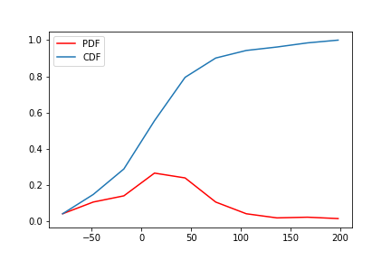
For the conventional distribution, the imply is outlined in Scipy because the variable loc, whereas the usual deviation is scale.
from scipy.stats import norm#norm.cdf(x, loc=mean_delay, scale=std_delay)
Now, what’s the likelihood of getting a delay for this connection? We have to exchange the random variable x with our delay threshold, thus a delay in seconds larger than 0 (the orange space beneath).

Furthermore, since we’re in search of P(x>0), and the CDF provides us P(x≤x), we should compute 1- P(x≤0).
from scipy.stats import normproba = norm.cdf(0, loc=mean_delay, scale=std_delay)
final_proba = 1 - proba
final_proba: 0.5641598241281299
As we will see, there can be a likelihood of 56% of getting a delay on this connection. After all, this considers any delay larger than 0 seconds. To additional enhance the evaluation, we might ask what the likelihood of getting greater than a 1-minute delay is.
from scipy.stats import normproba = norm.cdf(60, loc=mean_delay, scale=std_delay)
final_proba = 1 - proba
final_proba: 0.1774974181545348
As we will see, the likelihood is now solely 17%.
5. Conclusion
With this publish, I wished to point out you how one can apply information science to mannequin a simple downside corresponding to delay likelihood on an actual dataset. We began by gathering the delays at a given connection, discovering its imply and commonplace deviation, and at last match it in a cumulative distributive perform to search out the likelihood of getting the delay.
The concept of writing about likelihood distributions in delays comes from a undertaking I did in a course at EPFL during which we needed to construct a stochastic route planner for the Zürich Space (Switzerland). You’ll be able to see the app we did at this hyperlink and our GitHub repository right here. When you have any questions or feedback, be happy to attach with me on LinkedIn.
