
Enhance your matplotlib figures with these easy steps

Matplotlib is among the hottest knowledge visualisation libraries accessible inside Python. It’s usually the primary knowledge visualisation library that you just come throughout when studying python. Despite the fact that you may generate figures with just a few strains of code, the plots which are created are sometimes poor, visually unappealing and uninformative.
To fight this, we are able to improve the communication energy of the figures with just a few additional strains of code. Inside this text, we’ll cowl how we are able to go from a fundamental matplotlib scatter plot to 1 that’s extra visually interesting and extra informative to the top person/reader.

Within the following examples of how a scatter plot will be enhanced inside matplotlib we will likely be utilizing a subset of a bigger dataset that was used as a part of a Machine Studying competitors run by Xeek and FORCE 2020 (Bormann et al., 2020). It’s launched below a NOLD 2.0 licence from the Norwegian Authorities, particulars of which will be discovered right here: Norwegian Licence for Open Authorities Information (NLOD) 2.0.
The complete dataset will be accessed on the following hyperlink: https://doi.org/10.5281/zenodo.4351155.
For this tutorial, we might want to import each matplotlib and pandas.
The info is then learn right into a dataframe utilizing the pandas technique read_csv() . We may also calculate a density porosity column which we will likely be utilizing to plot towards neutron porosity.
import pandas as pd
import matplotlib.pyplot as pltdf = pd.read_csv('knowledge/Xeek_Well_15-9-15.csv')df['DPHI'] = (2.65 - df['RHOB'])/1.65df.describe()
Once we run the above code we get again the next abstract of the info with our new DPHI column.

After the info has been efficiently loaded, we are able to create our first scatter plot. To do that we’re going to plot neutron porosity (NPHI) on the x-axis and density porosity (DPHI) on the y-axis.
We may also set the determine dimension to 10 x 8.
plt.determine(figsize=(10,8))plt.scatter(df['NPHI'], df['DPHI'])

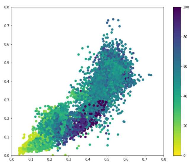
With these two strains of code, we get the above plot. Appears very bland, doesn’t it? Let’s add some color to make it extra visually interesting and to permit us to realize some perception into the info.
To try this we’re going to color the info by gamma ray (GR) and set the color vary between 0 and 100 (vmin and vmax parameters).
We might want to show the color bar through the use of plt.colorbar() .
Lastly, we’ll set the x and y limits of the chart to go from 0 to 0.8 by calling upon plt.xlim() and plt.ylim(). This may make each axes begin from 0 and go to a most of 0.8.
plt.determine(figsize=(10,8))plt.scatter(df['NPHI'], df['DPHI'], c=df['GR'], vmin=0, vmax=100, cmap='viridis_r')
plt.xlim(0, 0.8)
plt.ylim(0, 0.8)
plt.colorbar()
The color map we’re utilizing is Viridis in reverse. This color map offers a pleasant distinction between excessive and low values, while sustaining uniformity and being color blind pleasant.
Once we run the above code, we get again the next plot.
If you wish to discover out extra about selecting color maps and why some color maps will not be appropriate for everybody, then I extremely advocate testing this video right here:
The subsequent change we’ll make is to take away the black field surrounding the plot. Both sides of this field known as a backbone. Eradicating the highest and proper sides helps make our plot cleaner and extra visually interesting.
We are able to take away the proper and high axis by calling upon plt.gca().spines[side].set_visible(False) the place aspect will be high, proper, left or backside.
plt.determine(figsize=(10,8))plt.scatter(df['NPHI'], df['DPHI'], c=df['GR'], vmin=0, vmax=100, cmap='viridis_r')
plt.xlim(0, 0.8)
plt.ylim(0, 0.8)
plt.colorbar()plt.gca().spines['top'].set_visible(False)
plt.gca().spines['right'].set_visible(False)
After eradicating the spines, our plot seems cleaner and has much less muddle. Plus the color bar now appears like it’s a part of the plot reasonably than showing to be segmented.

When trying on the above scatter plot, we might know what every axis represents, however how are others going to know what this plot is about, what the colors characterize and what’s plotted towards what?
Including a title and axis labels to our plot is an important a part of creating efficient visualisations. These can merely be added through the use of:plt.xlabel , plt.ylabel, and plt.title. Inside every of those we go within the textual content we wish to seem and any font attributes equivalent to font dimension.
Additionally, it’s good apply to incorporate the models of measurement within the label. This helps readers to know the plot higher.
plt.determine(figsize=(10,8))plt.scatter(df['NPHI'], df['DPHI'], c=df['GR'], vmin=0, vmax=100, cmap='viridis_r')
plt.xlim(0, 0.8)
plt.ylim(0, 0.8)
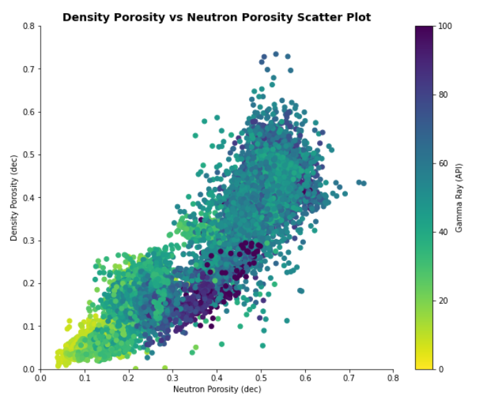
plt.colorbar(label='Gamma Ray (API)')plt.gca().spines['top'].set_visible(False)
plt.gca().spines['right'].set_visible(False)plt.title('Density Porosity vs Neutron Porosity Scatter Plot', fontsize=14, fontweight='daring')
plt.xlabel('Neutron Porosity (dec)')
plt.ylabel('Density Porosity (dec)')
plt.present()
Once we run the above code we get the next plot. Instantly we all know what’s plotted on the axes, what the chart is about and what the color vary represents.
Relying on the aim of the plot, we might wish to add a grid to in order that readers of the chart can visually and simply navigate the plot. That is particularly vital if we wish to quantitively extract values from the plot. Nevertheless, there are occasions when grid strains are thought-about “junk” and they’re greatest left off. For instance, when you simply wish to present normal tendencies inside a dataset and don’t need the reader to focus an excessive amount of on the uncooked values.
On this instance, we’ll add some faint gridlines in order that they don’t detract an excessive amount of from the info. To do that we have to add in plt.grid() to our code.
plt.determine(figsize=(10,8))plt.scatter(df['NPHI'], df['DPHI'], c=df['GR'], vmin=0, vmax=100, cmap='viridis_r')
plt.xlim(0, 0.8)
plt.ylim(0, 0.8)
plt.colorbar(label='Gamma Ray (API)')plt.gca().spines['top'].set_visible(False)
plt.gca().spines['right'].set_visible(False)plt.title('Density Porosity vs Neutron Porosity Scatter Plot', fontsize=14, fontweight='daring')
plt.xlabel('Neutron Porosity (dec)')
plt.ylabel('Density Porosity (dec)')plt.grid()
plt.present()
Nevertheless, after we do that we’ll discover that the grid strains seem on high of our plot, and it doesn’t look visually interesting.

To plot the grid strains behind, we have to transfer the plt.grid() line in order that it’s earlier than the decision to plt.scatter() and add within the parameter for zorder. This controls the order by which elements of the chart are plotted. It must be famous that these values are relative to different objects on the plot.
For the grid we wish the zorder worth to be lower than the worth we use for the scatter plot. On this instance, I’ve set the zorder to 1 for the grid and a pair of for the scatter plot.
Moreover, we’ll add in just a few extra parameters for the grid, particularly colour which controls the color of the grid strains and alpha which controls the transparency of the strains.
plt.determine(figsize=(10,8))
plt.grid(colour='lightgray', alpha=0.5, zorder=1)plt.scatter(df['NPHI'], df['DPHI'], c=df['GR'], vmin=0, vmax=100, cmap='viridis_r', zorder=2)
plt.xlim(0, 0.8)
plt.ylim(0, 0.8)
plt.colorbar(label='Gamma Ray (API)')plt.gca().spines['top'].set_visible(False)
plt.gca().spines['right'].set_visible(False)plt.title('Density Porosity vs Neutron Porosity Scatter Plot', fontsize=14, fontweight='daring')
plt.xlabel('Neutron Porosity (dec)')
plt.ylabel('Density Porosity (dec)')plt.present()
This returns a a lot nicer plot and the grid strains will not be too distracting.

Subsequent up is altering the scale of every of the info factors. In the meanwhile, the factors are comparatively giant and the place we have now a excessive density of knowledge the info factors can overlay one another.
One technique to counteract that is to scale back the scale of the info factors. That is achieved via the s parameter throughout the plt.scatter() operate. On this instance, we’ll set it to five.
plt.determine(figsize=(10,8))
plt.grid(colour='lightgray', alpha=0.5, zorder=1)plt.scatter(df['NPHI'], df['DPHI'], c=df['GR'], vmin=0, vmax=100, zorder=2, s=5, cmap='viridis_r')
plt.xlim(0, 0.8)
plt.ylim(0, 0.8)
plt.colorbar(label='Gamma Ray (API)')plt.gca().spines['top'].set_visible(False)
plt.gca().spines['right'].set_visible(False)plt.title('Density Porosity vs Neutron Porosity Scatter Plot', fontsize=14, fontweight='daring')
plt.xlabel('Neutron Porosity (dec)')
plt.ylabel('Density Porosity (dec)')
plt.present()
Once we run this code, we are able to see extra of the variation throughout the knowledge, and a greater thought of some extent’s true place.

When creating knowledge visualisations there are sometimes occasions after we wish to draw the reader’s consideration to a particular focal point. This might embody anomalous knowledge factors or key outcomes.
So as to add an annotation we are able to use the next line:
plt.annotate('Textual content We Need to Show', xy=(x,y), xytext=(x_of_text, y_of_text)
The place xy is the purpose on the chart we wish to level to and xytext is the place of the textual content.
If we needed to, we may additionally embody an arrow level from the textual content to the purpose on the chart. That is helpful if the textual content annotation is additional away from the purpose in query.
To additionally additional spotlight some extent or add one the place some extent doesn’t exist, we are able to add one other scatter plot on high of the prevailing one and go in a single x and y worth, and corresponding colors and elegance.
plt.determine(figsize=(10,8))plt.grid(colour='lightgray', alpha=0.5, zorder=1)plt.scatter(df['NPHI'], df['DPHI'], c=df['GR'], vmin=0, vmax=100, cmap='viridis_r',
zorder=2, s=5)
plt.xlim(0, 0.8)
plt.ylim(0, 0.8)
plt.colorbar(label='Gamma Ray (API)')plt.gca().spines['top'].set_visible(False)
plt.gca().spines['right'].set_visible(False)plt.title('Density Porosity vs Neutron Porosity Scatter Plot', fontsize=14, fontweight='daring')
plt.xlabel('Neutron Porosity (dec)')
plt.ylabel('Density Porosity (dec)')plt.scatter(0.42 ,0.17, colour='crimson', marker='o', s=100, zorder=3)
plt.annotate('Shale Level', xy=(0.42 ,0.17), xytext=(0.5, 0.05),
fontsize=12, fontweight='daring',
arrowprops=dict(arrowstyle='->',lw=3), zorder=4)plt.present()
When this code is run we get the next plot again. We are able to see that we have now a possible shale level highlighted on a plot by a crimson circle and a clear annotation with an arrow pointing to it.

Be aware that the purpose chosen is only for highlighting functions and {that a} extra detailed interpretation could be wanted to establish the true shale level inside this knowledge.
If there’s a complete space on a plot that we wish to spotlight, we are able to add a easy rectangle (or one other form) to shade that area.
For this, we have to import Rectangle from matplotlib.patches after which name upon the next line.
plt.gca().add_patch(Rectangle((x_position, y_position), width, peak, alpha=0.2, colour='yellow'))
The x_position and y_position characterize the decrease left nook of the rectangle. From there the width and peak are added.
We are able to additionally add in some textual content indicating what that space represents:
plt.textual content(x_position, y_position, s='Textual content You Need to Show, fontsize=12, fontweight='daring', ha='middle', colour='gray')
ha is used to place the textual content horizontally. Whether it is set to centre, then x_position and y_position characterize the centre of the textual content string. Whether it is set to left, then the x_position and y_position characterize the left-hand fringe of that textual content string.
from matplotlib.patches import Rectangleplt.determine(figsize=(10,8))plt.grid(colour='lightgray', alpha=0.5, zorder=1)plt.scatter(df['NPHI'], df['DPHI'], c=df['GR'], vmin=0, vmax=100, cmap='viridis_r',
zorder=2, s=5)
plt.xlim(0, 0.8)
plt.ylim(0, 0.8)
plt.colorbar(label='Gamma Ray (API)')plt.gca().spines['top'].set_visible(False)
plt.gca().spines['right'].set_visible(False)plt.title('Density Porosity vs Neutron Porosity Scatter Plot', fontsize=14, fontweight='daring')
plt.xlabel('Neutron Porosity (dec)')
plt.ylabel('Density Porosity (dec)')plt.scatter(0.42 ,0.17, colour='crimson', marker='o', s=100, zorder=3)
plt.annotate('Shale Level', xy=(0.42 ,0.17), xytext=(0.5, 0.05),
fontsize=12, fontweight='daring',
arrowprops=dict(arrowstyle='->',lw=3), zorder=4)plt.textual content(0.6, 0.75, s='Attainable Washout Results', fontsize=12, fontweight='daring', ha='middle', colour='gray')plt.gca().add_patch(Rectangle((0.4, 0.4), 0.4, 0.4, alpha=0.2, colour='yellow'))plt.present()
This code returns the next plot, the place we have now our space highlighted.

Inside this quick tutorial, we have now seen how we are able to go from a fundamental scatter plot generated by matplotlib, to 1 that’s rather more readable and visually interesting. This exhibits that with just a little bit of labor, we are able to get a significantly better plot that we are able to share with others and simply get our story throughout.
We have now seen take away pointless muddle by eradicating the spines, including gridlines to assist with qualitative evaluation, including titles and labels to point out what we’re displaying, and highlighting key factors that we wish to carry to the reader’s consideration.
