
Simply including arrows, a number of axes, gradient fill, and extra
Once we begin studying knowledge visualization strategies with instruments like matplotlib, we typically begin with the only attainable plots for ease of coding. Nonetheless, as we start sharing our visualizations with others, it’s vital to customise our plots to craft our message and make all the pieces extra visually interesting.
Reasonably than create advanced code and spending hours to make a plot look “excellent,” we will drop in a few traces of code to make our plots extra practical and assist the info inform a narrative to our viewers.
Listed below are 4 fast ideas so as to add emphasis, performance, and visible enchantment to fundamental matplotlib line and bar plots:
The objective is to make standalone plots that may inform a narrative, whether or not you’re there to current the slides or not. Earlier than sharing a graph, you need to be considering “what conclusions do I need my viewers to attract from this?” and “what a part of the info do I actually need them to note?” To assist with this, we will use lists to customise numerous the tunable parameters that include bar plots. What was colour='blue' can turn out to be colour=['blue', 'red', ...] with every entry indicating what to do with every bar in our plot.
For example, a easy bar plot appears to be like one thing like this:
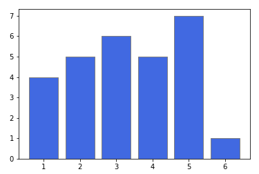
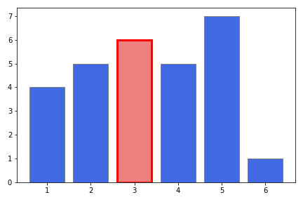
Nonetheless, if we needed to attract consideration to the third bar (for instance), we will do this by altering the colour, edgecolor, and linewidth inputs into lists:
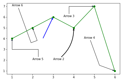
Line plots might be difficult so as to add emphasis. For line plots, easiest is normally greatest — including an arrow pointing to a selected knowledge level is a good way to drag the viewers’s eyes. Whereas matplotlib has a selected arrow operate, it’s fairly rigid and oddly difficult to get arrows to point out up “excellent”. A a lot less complicated and faster method to go is utilizing the annotate operate. Right here, we get a lot of performance that’s fairly intuitive. Our two important variables xytext and xy inform the place the arrow begins and ends, respectively. The xytext can also be the top of the arrow the place textual content can be positioned, ought to we select to label the arrow (however we don’t need to!).
We will modify the arrow properties utilizing arrowprops=dict(), whereby we will use the usual keys like colour, linewidth, and extra. That will get you easy, straight traces — however issues can get extra fascinating from there. We will modify the form of the arrowhead with arrowstyle (full checklist right here), and likewise deviate from a straight arrow path. connectionstyle is available in three important flavors —
arc3— curved path the place the diploma of curvature is about in radians (rad). Play with constructive and unfavorableradvalues to show your curve from concave to convex. In a line plot with straight connections, including a little bit of curvature to the arrow path positively helps it get observed.angle— segments of the road drawn at a specified angles (angleA,angleB). The tactic is sensible sufficient to make nearly no matter angles you select join between your textual content andxycoordinates.bar— segments are stored at 90 diploma bends of one-another, although your complete arrow might be primarily based on a standard angle. By taking part in withfractionright here we’re altering the place the flip is in relation to the endpoints. Strive unfavorable values on the code under and see what occurs!
Given the big variety of forms of arrows you may create, it’s greatest to experiment with the parameters to get precisely what you’re on the lookout for. Right here’s an instance with 6 totally different arrows utilized to our plot to assist visualize what is feasible.
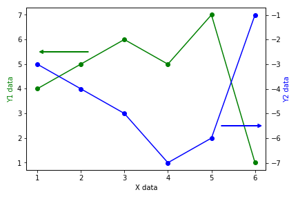
Overlaying a number of columns of knowledge on a single plot can drive conclusions in regards to the relationships between them. Nonetheless, it’s uncommon that each columns function on the identical numerical scale, inflicting scaling points the place one of many traces hovers close to the axis. To construct a secondary y-axis, we use the twinx() operate to create a secondary y-axis that shares the identical x-axis. This secondary axis will routinely be positioned on the far proper, and can be auto-scaled primarily based on the info fed to this ax merchandise. It is very important use colour to assist our viewers perceive which plot is related to every axis. To essentially drive the purpose dwelling, arrows might be added utilizing the tips we simply discovered.
Aspect word: including a secondary y-axis can be simply performed in native pandas, utilizing the secondary_y = True attribute, yielding an virtually an identical outcome. For those who’re curious, the code is right here and the ensuing plot is right here.
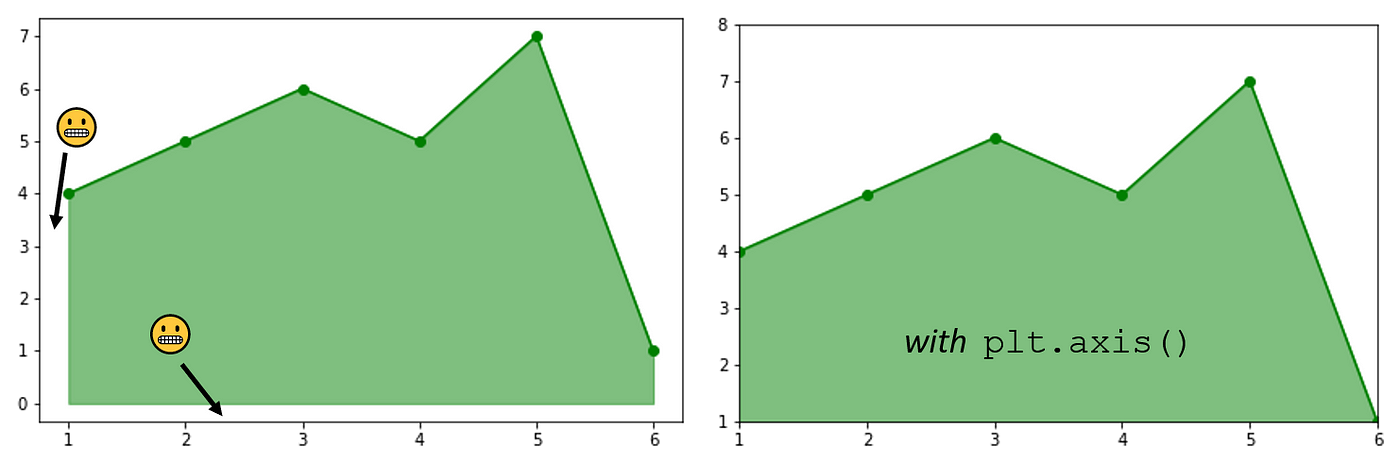
We will additionally add emphasis and basic visible enchantment to our line plots by filling within the area under the road. It is a fast addition utilizing the fill_between() operate the place we point out the x vary that we would like it to fill, and the 2 “traces” that we’d prefer to fill between. On this case, we’re eager to fill between the info and the underside of the plot (y=0 on this case). It’s additionally a good suggestion to set the plot space to match your knowledge with plt.axis(), in any other case the colour gained’t proceed to fill exterior of your knowledge vary, leaving unpleasant white areas in your plot.
We will push the boundaries a bit additional — turning our fill right into a colour gradient. On this case, we have now to get artistic. imshow() is nice for including gradients, nevertheless it historically does it over our complete plot space. To beat this, we add a gradient with imshow(), then use fill_between() to paint all the pieces above our line white. imshow() is a bit difficult to get off the bottom, and I’ve gone into extra depth of it in considered one of my prior articles linked right here. Nonetheless, the straightforward model has us set the vary of the colour map we’re utilizing in X — right here we select a vertical colour gradient utilizing the underside 80% of the cm.Blues colour map with [[0.8, 0.8],[0,0]]. (The same horizontal gradient might be achieved like this: X=[[0,0.8][0,0.8]]).
We additionally set the extent of the imshow() fill, successfully setting the bounding field for this gradient picture fill. We will set the values manually, or use our min() and max() capabilities on our knowledge collection. These might be merely augmented to increase the plot area additional down. Lastly, we set the higher certain of the plot space within the fill_between() operate, as we now go from our knowledge to a the highest of the plot (outlined right here as df.b.max()+0.5 ).

Taking what we’ve discovered, we will now mix our strategies to affix two line plots utilizing a secondary axis, whereas additionally including fill and annotating an vital level with an arrow.
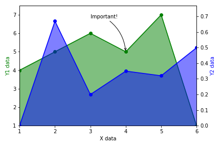
With a number of fast changes to our code we will add each emphasis and visible enchantment to our matplotlib plots. Emphasised plots allow our knowledge to talk for itself and may immediately drive others to give attention to the info factors that we suppose are price taking note of. Fortunately, we will attain this objective with only a few traces of code!
As at all times, your complete code walk-through pocket book might be snagged from my github. Please observe me should you discovered this handy! Cheers, and joyful coding on the market.
