3D Machine Studying Course: Level Cloud Semantic Segmentation

Full python tutorial to create supervised studying AI methods for semantic segmentation of unstructured 3D LiDAR level cloud knowledge

Having the abilities and the data to assault each side of level cloud processing opens up many concepts and growth doorways. 🤖 It is sort of a toolbox for 3D analysis creativity and growth agility. And on the core, there’s this unimaginable Synthetic Intelligence house that targets 3D scene understanding. 🏡

It’s significantly related as a result of its significance for a lot of purposes, comparable to self-driving automobiles, autonomous robots, 3D mapping, digital actuality, and the Metaverse. And in case you are an automation geek like me, it’s laborious to withstand the temptation to have new paths to reply these challenges!

This tutorial goals to present you what I contemplate the important footing to just do that: the data and code abilities for creating 3D Level Cloud Semantic Segmentation methods.

However really, how can we apply semantic segmentation? And the way difficult is 3D Machine Studying?

Let me current a transparent, in-depth 201 hands-on course targeted on 3D Machine Studying. On this tutorial, I’ll cowl exactly what’s 3D Machine Studying and the way we are able to leverage environment friendly python code to provide semantic predictions for unstructured 3D level clouds.

Desk of Contents3D Scene Notion
✔️ 3D Sensors
✔️ 3D Scene Understanding
✔️ ClassificationSemantics Addition Strategies for 3D knowledge
✔️ 3D Object Detection
✔️ 3D Semantic Segmentation
✔️ 3D Occasion Segmentation3D Predictions with Supervised studying3D Python Workflow
✔️ Step 1: Definition and Knowledge Curation
✔️ Step 2. Setting Set-up
✔️ Step 3. 3D Function Engineering
✔️ Step 4. 3D Machine Studying
✔️ Step 5. Efficiency EvaluationConclusion

Allow us to dive proper in! 🤿

Recognizing 3D objects in LiDAR (which stands for Gentle Detection and Ranging) is a superb problem because of the complicated nature of the 3D captured knowledge. The uncooked level clouds acquired through 3D scanning methods are unstructured, unrefined, unordered, and liable to irregular sampling making the 3D Scene understanding process difficult. So, what ought to we do? Is it possible in any respect? Ha, that’s what we like! A real problem!😉

👀 3D sensors

Allow us to begin with the enter to our system. 3D sensors (LiDAR, Photogrammetry, SAR, RADAR, and Depth-Sensing Cameras) will primarily describe a scene by many 3D factors in house. These can then host helpful info and allow machine studying methods that use these inputs (E.g. autonomous automobiles and robots) to function in the true world and create an improved Metaverse expertise. Okay, so we’ve a base enter from the sensory info, what’s subsequent?

🏕️ 3D Scene Understanding

You guessed it: Scene understanding. It describes the method that perceives, analyzes, and elaborates an interpretation of the 3D scene noticed by a number of of those sensors (The Scene may even be dynamic!). Down the road, this process consists primarily in matching sign info from the sensors observing the Scene with “fashions” we use to know the Scene. Relying on how fluffy is the magic 🧙‍♂️, the fashions will allow a pertinent “scene understanding”. On a low-level view, methods are extracting and including semantics from the enter knowledge characterizing a scene. Do these methods have a reputation?

🦘/🐈‍⬛ Classification

Effectively, what we classically cowl in 3D Scene Understanding framework is the duty of Classification. The principle purpose of this step is to know the enter knowledge and to interpret what totally different elements of the sensor knowledge are. For instance, we’ve some extent cloud of an outside scene, comparable to a freeway, collected by an autonomous robotic or a automobile. The purpose of Classification is to determine the principle constituting elements of the Scene, so understanding which elements of this level cloud are roads, which elements are buildings, or the place are the people. It’s, on this sense, an total class that goals at extracting particular semantic that means from our sensor knowledge. And from there, we need to add the semantics at totally different granularities. 👇

As you possibly can see beneath, including semantics to the 3D scenes could be accomplished by varied methods. These aren’t essentially impartial designs, and we are able to typically depend on a hybrid meeting when wanted.

Let me describe with a bit extra texture every of those methods.

📦 3D Object Detection

The primary one would enclose the 3D object detection methods. It’s a very important element for lots of purposes. Principally, it permits the system to seize objects’ sizes, orientations, and positions on the earth. Because of this, we are able to use these 3D detections in real-world situations comparable to Augmented Actuality Purposes, Self-driving automobiles, or robots which understand the world by restricted spatial/visible cues. Good, 3D cubes that comprise totally different objects. However what if we need to fine-tune the contours of objects?

🏘️ 3D Semantic Segmentation

Effectively, that is the place we’ll assault the issue with Semantic Segmentation methods. It is likely one of the most difficult duties that assigns semantic labels to each base unit (i.e., each level in some extent cloud) that belongs to the objects of curiosity. Primarily, 3D semantic segmentation purpose at higher delineation of objects current in a scene. A 3D Bounding Field Detection on steroïd if you’ll. Due to this fact, it means having semantic info per level. We will go deep there. However nonetheless, a limitation stays: we can not straight deal with totally different objects per class (class) we assault. Do we’ve methods for this as nicely?

🏠 3D Occasion Segmentation

Sure! And it’s known as 3D occasion segmentation. It has even broader purposes, from 3D notion in autonomous methods to 3D reconstruction in mapping and digital twinning. For instance, we may think about a listing robotic that identifies chairs, is ready to rely what number of there are, after which transfer them by greedy them by the fourth leg. Reaching this purpose requires distinguishing totally different semantic labels in addition to totally different situations with the identical semantic label. I might qualify Occasion segmentation as a Semantic Segmentation step on Mega-Steroïds 😁.

Now that you’ve got a base understanding and a taxonomy of the present strategies for various outputs, the query stays: Which technique ought to we comply with to inject semantic predictions? 🤔

If you’re nonetheless there, then you’ve got handed the mumble bumble 3D charabia, and are prepared to know the mission by its uni-horn.🦄 We need to extract semantic info and inject it into our 3D knowledge within the type of level clouds. To just do that, we’ll deepen one technique that helps us derive such info from the sensor. We’ll concentrate on one algorithm household, supervised studying strategies — versus unsupervised strategies proven beneath.

With supervised studying strategies, we primarily present explicit categorized examples to the methods from the previous. It implies that we want someway to label these examples. And for this, you’ve got the next tutorial:

Then, we use the labels for every thought of factor within the Scene to have the ability to predict labels about future knowledge. Thus the purpose is to have the ability to infer knowledge that has not been seen but, as illustrated beneath.

However how can we assess how nicely the skilled mannequin performs? Is a visible evaluation sufficient (is that this an precise query? 🙃)

Effectively, a visible evaluation — allow us to name it qualitative evaluation — is just one a part of the reply. The opposite massive block is held by a quantitative evaluation evaluated utilizing a wide range of metrics that may spotlight particular performances of our methodology. It’s going to assist us characterize how nicely a selected classification system works and provides us instruments to decide on between totally different classifiers for the appliance.

And now, the (mild) concept is over! Allow us to dive right into a enjoyable python code implementation in 5 steps🤲! I like to recommend having a superb 🫐 bowl.

Aerial LiDAR Level Cloud Dataset Sourcing

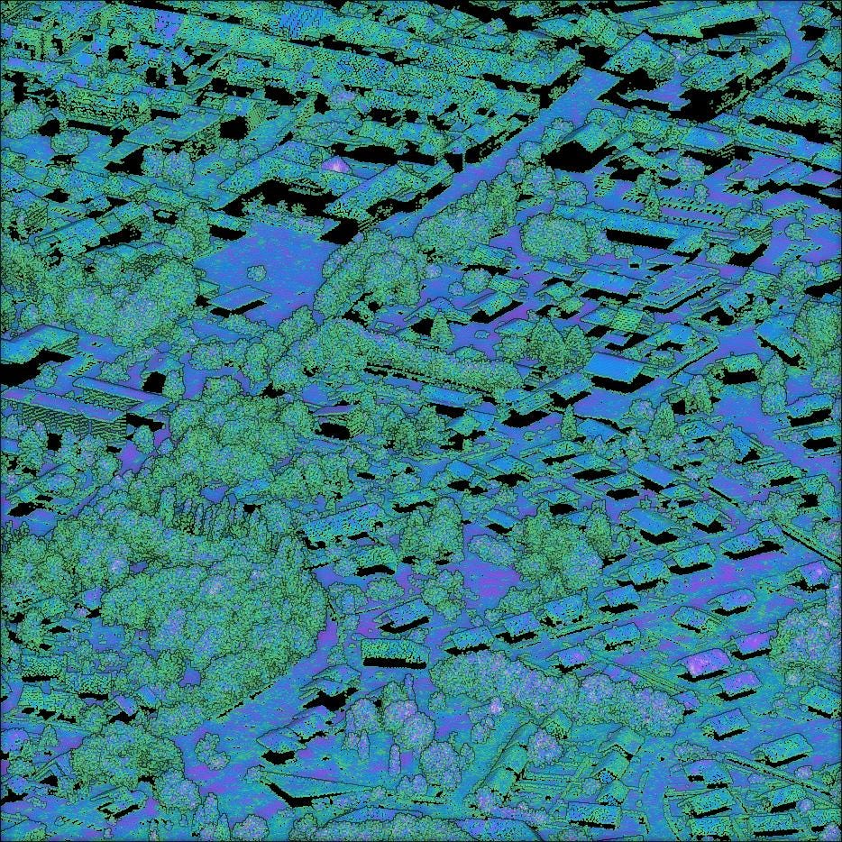
You understand the drill? Step one we make is to dive into the online and supply some enjoyable 3D knowledge! This time, I need to deep dive a French (sorry for being such a snob 😆) place to seek out chilled LiDAR datasets: The Nationwide Geography Institute (IGN) of France. With the LiDAR HD marketing campaign, France begins an OpenData gathering the place you may get crisp 3D level clouds of some areas of France! And on prime, some have labels that make it straightforward to not begin from scratch, as one can find within the hyperlink beneath.

However to make the tutorial easy, I went on the portal above, chosen the info overlaying a part of the town of Louhans (71), deleted the georeferencing info, computed some additional attributes (that I’ll clarify in one other tutorial 😜), after which made it obtainable in my Open Knowledge Drive Folder. The info you have an interest in are 3DML_urban_point_cloud.xyz and 3DML_validation.xyz. You possibly can leap on the Flyvast WebGL extract if you wish to visualize it on-line.

The general loop technique

I suggest to comply with a easy process that you would be able to rapidly replicate to coach a 3D machine studying mannequin and apply it to real-world purposes, as illustrated beneath.

🤓 Be aware: The technique is just a little extract from one of many paperwork given on the web programs I host on the 3D Geodata Academy. This tutorial will cowl steps 4 to eight + 10 + 11, the opposite ones coated in depth within the course, or by following one of many tutorials by this help hyperlink.

On this hands-on level cloud tutorial, I concentrate on environment friendly and minimal library utilization. For the sake of mastering python, we’ll do all of it with solely two libraries: Pandas, and ScikitLearn. And we’ll do wonders 😁. 5 strains of code to begin your script:

import pandas as pdfrom sklearn.model_selection import train_test_split
from sklearn.metrics import classification_reportfrom sklearn.ensemble import RandomForestClassifier
from sklearn.preprocessing import MinMaxScaler

🤓 Be aware: As you possibly can see, I import capabilities and modules from the libraries in several methods. For pandas, I take advantage of import module, which calls for much less upkeep of the import statements. Nonetheless, whenever you need extra management over which objects of a module could be accessed, I like to recommend utilizing from module import foo, which allows much less typing to make use of foo.

Good! from there, I suggest that we comparatively categorical our paths, separating the data_folder containing our datasets from the dataset title to change simply on the fly:

data_folder=”../DATA/”
dataset="3DML_urban_point_cloud.xyz"

Now, we are able to rapidly load the dataset within the pcd variable utilizing Pandas. And since the unique file shouldn’t be clear and accommodates NaN values, we’ll use the very useful dropna methodology inplace to make sure we begin with a filtered dataframe with solely full rows. Nonetheless, this implies we’ll drop some factors alongside the best way (<1% of information), however this time we’re okay with that.

pcd=pd.read_csv(data_folder+dataset,delimiter=' ')
pcd.dropna(inplace=True)

🤓 Be aware: The inplace argument set to True permits to straight substitute the python object as an alternative of constructing a dataframe copy.

To grasp what we do when utilizing Machine Studying frameworks, it’s important to perceive that we depend on characteristic units or vectors of options which can be variably consultant. In our method, the trick is to know very nicely the context during which we evolve and to be inventive with methods to engineer options that we consider might be wonderful descriptors of the variance in our knowledge. Or at the very least assist us distinguish between the lessons of curiosity.

I made a decision to create one other targeted tutorial on simply the preparatory steps to acquire such options. However for the sake of simplicity, I already computed a bunch of them for you, filtered with the first intention to be pertinent for subsequent semantic segmentation duties.

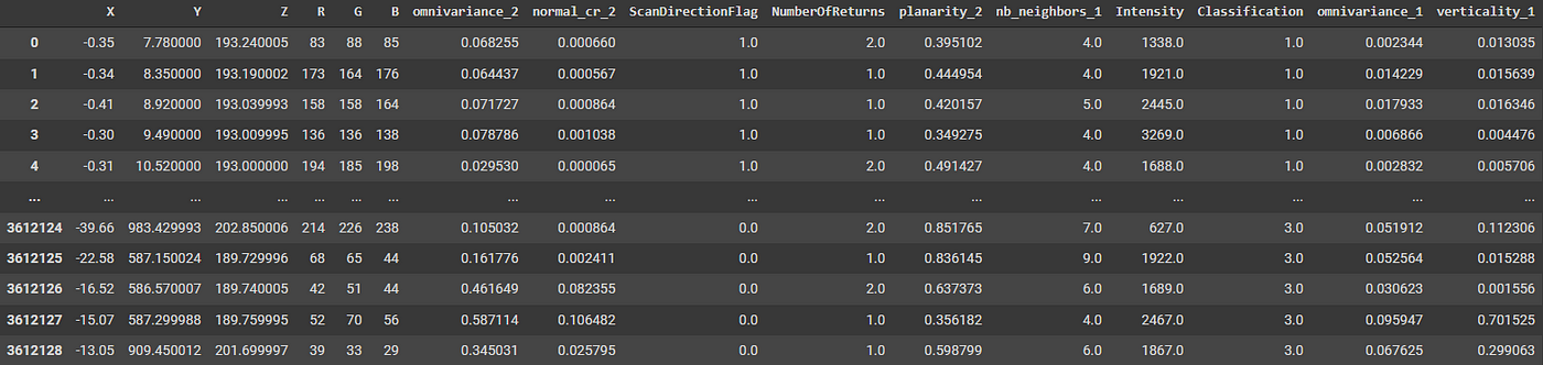
To get began on a strong base, we’ll set up our options between labels, i.e., what we’ll attempt to predict, and the options, i.e., what we’ll use to make our predictions. With Pandas, we are able to simply try this in two strains of code:

labels=pcd['Classification']options=pcd[['X','Y','Z','R','G','B']]

This dataframe structuration permits rapidly switching to a selected set of pertinent options with out utilizing numeric indexes. Thus be happy to return at this step and alter the options vector set.

Choosing the options

Function Choice is the strategy of lowering the enter variable fed to your mannequin by utilizing solely probably the most related ones and eliminating noise in knowledge. It’s the course of of selecting related options on your machine studying mannequin based mostly on the kind of downside you are attempting to resolve. If accomplished robotically, this falls beneath the AutoML technique of automating the duties of making use of machine studying to real-world issues.

You may have two instructions right here. You both go absolutely unsupervised (E.g., lowering correlations inside your options) or in a supervised trend (E.g., seeking to improve the ultimate rating of the mannequin after altering options and parameters).

For the sake of simplicity, we’ll manually alter the collection of our present characteristic vector by the supervised course: we’ll run experiments and alter if the outcomes aren’t ok. Prepared? 🙂

Getting ready the options

As soon as our preliminary characteristic vector is prepared, we are able to rush into processing!💨 or can we? Be cautious! Relying on the Machine Studying Mannequin we use, we could encounter some surprises! Certainly, allow us to take a easy state of affairs.

Allow us to think about that our chosen characteristic vector is the next:

options=pcd[['X','Y']]

Right here, if we might use that to coach our algorithm, then we might be caught to the seen vary, e.g., X various between 0 and 100. If, after coaching on this vary, the mannequin is fed with future knowledge with an identical distribution however a special vary, e.g., X from 1100 to 1200, then we may get catastrophic outcomes, even when it’s the identical dataset, simply having a translation in between. Certainly, for some fashions, the X worth, which is above 100, could make the mannequin predict an misguided worth, whereas if beforehand we ensured that we translated the info to the identical vary seen in coaching. The predictions would have higher possibilities of making sense.

I turned to the idea of characteristic scaling and normalization. It’s a essential a part of the info preprocessing stage, however I’ve seen many inexperienced persons overlook it (to the detriment of their machine studying mannequin). A mistake we won’t make! 💪

As a result of we’re in a spatial-heavy context, a great way of avoiding generalization issues is to scale back to what we name the Min-Max normalization. For this, we’ll use the MinMaxScaler operate:

from sklearn.preprocessing import MinMaxScaler
features_scaled = MinMaxScaler().fit_transform(options)

💡 Trace: The MinMaxScaler() transforms options by scaling and translating every characteristic individually to be within the given vary, e.g., between zero and one. In case your knowledge is generally distributed, then you might use StandardScaler.

3D Machine Studying Coaching set-up

Okay, we’ve a labels vector and a correct options vector. Now, we have to put together a set-up for the coaching section. For beginning, we’ll break up each vectors — whereas maintaining the correct index match between labels and options — to make use of a portion for coaching the machine studying mannequin and one other portion just for trying on the performances. We use 60% of the info for coaching, and 40% for trying on the performances, each taken from the identical distribution randomly. It’s made utilizing the train_test_split operate from scikitlearn:

X_train, X_test, y_train, y_test = train_test_split(features_scaled, labels, test_size=0.4)

🤓 Be aware: We use naming conventions when coping with knowledge for Machine Studying duties. X denotes the options (or knowledge) fed to a mannequin and y denotes the labels. Every is decomposed into _train or _test relying on their finality.

We then create a “classifier object” by:

rf_classifier = RandomForestClassifier()

🤓 Be aware: The classifier above is a Random Forest classifier. In a single sentence, it matches a number of determination tree classifiers on varied sub-samples of the options and makes use of averaging to enhance the predictive accuracy and management over-fitting. Compelling stuff 😁.

After classifier initialization, we match the classifier to the coaching knowledge to regulate its core parameters. This section is the coaching section, which might take some minutes relying on the hyperparameters (i.e., the parameters that outline the Machine Studying mannequin structure) that we used beforehand (variety of bushes, depth):

rf_classifier.match(X_train, y_train)

And on the finish, voilà! Now we have a skilled mannequin! Sure, it’s that straightforward! So it’s also that straightforward to take shortcuts. 😉

For the prediction section, whether or not you’ve got labels or not, it’s essential do the next:

rf_predictions = rf_classifier.predict(X_test)

you possibly can then visualize outcomes and variations with the next code block that may create three subplots: the 3D level cloud knowledge floor reality, the predictions, and the distinction between each:

fig, axs = plt.subplots(1, 3, figsize=(20,5))
axs[0].scatter(X_test['X'], X_test['Y'], c =y_test, s=0.05)
axs[0].set_title('3D Level Cloud Floor Fact')
axs[1].scatter(X_test['X'], X_test['Y'], c = rf_predictions, s=0.05)
axs[1].set_title('3D Level Cloud Predictions')
axs[2].scatter(X_test['X'], X_test['Y'], c = y_test-rf_predictions, cmap = plt.cm.rainbow, s=0.5*(y_test-rf_predictions))
axs[2].set_title('Variations')

and if you wish to try some metrics, we are able to print a classification report with a bunch of numbers utilizing the classification_report operate of scikit-learn:

print(classification_report(y_test, rf_predictions))

However ought to we not perceive what every metric means? 🤔

Performances and Metrics

We will use a number of quantitative metrics for assessing semantic segmentation and classification outcomes. I’ll introduce to you 4 metrics which can be very helpful for 3D level cloud semantic segmentation evaluation: precision, recall, F1-score, and total accuracy. All of them depend upon what we name true constructive and true unfavorable:

• True Optimistic (TP): Remark is constructive and is predicted to be constructive.
• False Destructive (FN): Remark is constructive however is predicted unfavorable.
• True Destructive (TN): Remark is unfavorable and is predicted to be unfavorable.
• False Optimistic (FP): Remark is unfavorable however is predicted constructive.

The General Accuracy is a common measure on all observations in regards to the classifier’s efficiency to foretell labels accurately. The precision is the power of the classifier to not label as constructive a pattern that’s unfavorable; the recall is intuitively the power of the classifier to seek out the entire constructive samples. Due to this fact, you possibly can see the precision as a superb measure to know in case your mannequin is exact and the recall to know with which exhaustivity you discover all objects per class (or globally). The F1-score could be interpreted as a weighted harmonic imply of the precision and recall, thus giving measure of how nicely the classifier performs with one quantity.

🤓 Be aware: Different international accuracy metrics aren’t acceptable analysis measures when class frequencies are unbalanced, which is the case in most situations, each in pure indoor and outside scenes, for the reason that dominant lessons bias them. Henceforth, the F1-score in our experiments signifies the common efficiency of a proposed classifier.

Mannequin Choice

It’s time to choose a selected 3D Machine Studying Mannequin. For this tutorial, I restricted the selection to 3 Machine Studying fashions: Random Forests, Ok-Nearest Neighbors, and a Multi-Layer Perceptron that falls throughout the Deep Studying class. To make use of them, we’ll first import the required capabilities with the next:

from sklearn.neighbors import RandomForestClassifier
rf_classifier = RandomForestClassifier()from sklearn.neighbors import KNeighborsClassifier
knn_classifier = KNeighborsClassifier()from sklearn.neural_network import MLPClassifier
mlp_classifier = MLPClassifier(solver='lbfgs', alpha=1e-5,hidden_layer_sizes=(15, 2), random_state=1)

Then, you simply have to switch XXXClassifier() within the following code block by the wished algorithm stack:

XXX_classifier = XXXClassifier()
XXX_classifier.match(X_train, y_train)
XXX_predictions = XXXclassifier.predict(X_test)
print(classification_report(y_test, XXX_predictions, target_names=['ground','vegetation','buildings']))

🤓 Be aware: For simplicity, I handed to the classification_report the checklist of the tree lessons that correspond to the bottom, vegetation, and buildings current in our datasets.

And now, to the checks section on utilizing the three classifiers above with the next parameters:

Practice / Take a look at Knowledge: 60%/40% 
Variety of Level within the take a look at set: 1 351 791 / 3 379 477 pts
Options chosen: ['X','Y','Z','R','G','B'] - With Normalization

Random Forests

We begin with Random Forests. Some kind of magical bushes conjuration by an ensemble algorithm that mixes the a number of determination bushes to present us the ultimate consequence: an total accuracy of 98%, based mostly on a help of 1.3 million factors. It’s additional decomposed as follows:

╔════════════╦══════════════╦══════════╦════════════╦═════════╗
║  lessons   ║    precision ║   recall ║   f1-score ║ help ║
╠════════════╬══════════════╬══════════╬════════════╬═════════╣
║ floor     ║         0.99 ║     1.00 ║       1.00 ║  690670 ║
║ vegetation ║         0.97 ║     0.98 ║       0.98 ║  428324 ║
║ buildings  ║         0.97 ║     0.94 ║       0.96 ║  232797 ║
╚════════════╩══════════════╩══════════╩════════════╩═════════╝

🤓 Be aware: Nothing a lot to say right here, relatively than it gives spectacular outcomes. The bottom factors are nearly completely categorized: the 1.00 recall implies that all factors that belong to the bottom had been discovered, and the 0.99 precision means that there’s nonetheless a tiny margin of enchancment to make sure no False Optimistic. Auqlitqtivelym ze see that the errors are distributed a bit in all places, which could possibly be problematic if this must be corrected manually.

Ok-NN

The Ok-Nearest Neighbors classifier makes use of proximity to make predictions about a person knowledge level grouping. We receive a 91% international accuracy, additional decomposed as follows:

╔════════════╦══════════════╦══════════╦════════════╦═════════╗
║  lessons   ║    precision ║   recall ║   f1-score ║ help ║
╠════════════╬══════════════╬══════════╬════════════╬═════════╣
║ floor     ║         0.92 ║     0.90 ║       0.91 ║  690670 ║
║ vegetation ║         0.88 ║     0.91 ║       0.90 ║  428324 ║
║ buildings  ║         0.92 ║     0.92 ║       0.92 ║  232797 ║
╚════════════╩══════════════╩══════════╩════════════╩═════════╝

🤓 Be aware: The outcomes are decrease than Random Forests, which is anticipated as a result of we’re extra topic to native noise within the present vector house. Now we have a homogeneous precision/recall steadiness over all lessons, which is an effective signal that we keep away from overfitting problematics. No less than within the present distribution 😁.

3D Deep Studying with a Multi-Layer Perceptron

The Multi-Layer Perceptron (MLP) is a Neural Community algorithm that learns linear and non-linear knowledge relationships. The MLP requires tuning a number of hyperparameters, such because the variety of hidden neurons, layers, and iterations, making it laborious to get excessive performances out of the field. For instance, with the hyperparameters set, we’ve a worldwide accuracy of 64% additional decomposed as follows:

╔════════════╦══════════════╦══════════╦════════════╦═════════╗
║  lessons   ║    precision ║   recall ║   f1-score ║ help ║
╠════════════╬══════════════╬══════════╬════════════╬═════════╣
║ floor     ║         0.63 ║     0.76 ║       0.69 ║  690670 ║
║ vegetation ║         0.69 ║     0.74 ║       0.71 ║  428324 ║
║ buildings  ║         0.50 ║     0.13 ║       0.20 ║  232797 ║
╚════════════╩══════════════╩══════════╩════════════╩═════════╝

🤓 Be aware: On objective, the MLP metrics present instance of what’s thought of poor metrics. Now we have an accuracy rating decrease than 75%, which is usually the first-hand metric to focus on, after which we see vital variations between Intra and inter lessons. Notably, the buildings class may be very removed from being strong, and we could have an overfitting downside. Visually, that is discovered as nicely, as we are able to see that it’s the major supply of confusion in regards to the Deep Studying mannequin.

At this step, we won’t enhance by characteristic choice, however we may all the time have this risk. We determined to go together with the perfect performing mannequin at this step, the Random Forest method. And now, we’ve to analyze if the at present skilled mannequin performs nicely beneath difficult unseen situations, prepared? 😄

Now it will get difficult. Taking a look at what we’ve above, we could possibly be nicely beneath large hassle if we wished to scale the present mannequin to real-world purposes that stretch the scope of the present pattern dataset. So allow us to go right into a fully-fledged deployment of the mannequin.

The validation dataset

It’s a essential idea that I suggest to make sure avoiding overfitting problematics. As a substitute of utilizing solely a coaching dataset and a testing dataset from the identical distribution, I consider it is important to have one other unseen dataset with totally different traits to measure real-world performances. As such, we’ve:

• Coaching Knowledge: The pattern of information used to suit the mannequin.
• Take a look at Knowledge: The pattern of information used to offer an unbiased analysis of a mannequin fitted on the coaching knowledge however used to tune the mannequin hyperparameters and have vector. The analysis thus turns into a bit biased as we used that to tune enter parameters.
• Validation Knowledge: The uncorrelated pattern of information is used to offer an unbiased analysis of a remaining mannequin fitted to the coaching knowledge.

Under are some further clarifying notes:

• The take a look at dataset may play a task in different types of mannequin preparation, comparable to characteristic choice.
• The ultimate mannequin could possibly be match on the mixture of the coaching and validation datasets, however we determined to not.

The chosen validation knowledge is from the town of Manosque (04), which presents a special city context, with totally different topography and a broadly totally different city context, for instance, as seen beneath. This fashion, we improve the problem of dealing with Generalization 😆.

You possibly can obtain the 3DML_validation.xyz dataset from my Open Knowledge Drive Folder if not accomplished already. As defined beneath, additionally, you will discover the labels to review metrics and potential beneficial properties on the totally different iterations I made.

Bettering the Generalization outcomes

Our purpose might be to examine the validation dataset outcomes and see if we bypassed some prospects.

First, we import the validation knowledge in our script with the next three strains of code:

val_dataset="3DML_validation.xyz"
val_pcd=pd.read_csv(data_folder+dataset,delimiter=' ')
val_pcd.dropna(inplace=True)

Then, we put together the characteristic vector to have the identical options because the one used to coach the mannequin: no much less, no extra. We additional normalize our characteristic vector to be in the identical situation as our coaching knowledge.

val_labels=val_pcd['Classification']
val_features=val_pcd[['X','Y','Z','R','G','B']]
val_features_scaled = MinMaxScaler().fit_transform(val_features)

Then we apply the already skilled mannequin to the validation knowledge, and we print the outcomes:

val_predictions = rf_classifier.predict(val_features_scaled)
print(classification_report(val_labels, val_predictions, target_names=['ground','vegetation','buildings']))

That leaves us with a remaining accuracy of 54% for 3.1 million factors (towards 98% for the take a look at knowledge containing 1.3 million factors) current within the validation dataset. It’s decomposed as follows:

╔════════════╦══════════════╦══════════╦════════════╦═════════╗
║  lessons   ║    precision ║   recall ║   f1-score ║ help ║
╠════════════╬══════════════╬══════════╬════════════╬═════════╣
║ floor     ║         0.65 ║     0.16 ║       0.25 ║ 1188768 ║
║ vegetation ║         0.59 ║     0.85 ║       0.70 ║ 1315231 ║
║ buildings  ║         0.43 ║     0.67 ║       0.53 ║  613317 ║
╚════════════╩══════════════╩══════════╩════════════╩═════════╝

You simply witnessed the true darkish facet energy of Machine Studying: overfitting a mannequin to a pattern distribution and having large hassle generalizing. As a result of we’ve already ensured that we normalized our knowledge, we are able to examine the likelihood that this low-performance habits could also be as a result of options not distinctive sufficient. I imply, we used a few of the most typical/primary options. So allow us to enhance with a greater characteristic choice, for instance, the one beneath:

options=pcd[['Z','R','G','B','omnivariance_2','normal_cr_2','NumberOfReturns','planarity_2','omnivariance_1','verticality_1']]val_features=val_pcd[['Z','R','G','B','omnivariance_2','normal_cr_2','NumberOfReturns','planarity_2','omnivariance_1','verticality_1']]

Nice, we now restart the coaching section on the take a look at knowledge, we try the efficiency of the mannequin, after which we try the way it behaves on the validation dataset:

features_scaled = MinMaxScaler().fit_transform(options)
X_train, X_test, y_train, y_test = train_test_split(features_scaled, labels, test_size=0.3)
rf_classifier = RandomForestClassifier(n_estimators = 10)
rf_classifier.match(X_train, y_train)
rf_predictions = rf_classifier.predict(X_test)
print(classification_report(y_test, rf_predictions, target_names=['ground','vegetation','buildings']))val_features_scaled = MinMaxScaler().fit_transform(val_features)
val_rf_predictions = rf_classifier.predict(val_features_scaled)
print(classification_report(val_labels, val_rf_predictions, target_names=['ground','vegetation','buildings']))

Allow us to examine the outcomes. We now have 97% accuracy on the take a look at knowledge, additional decomposed as follows:

╔════════════╦══════════════╦══════════╦════════════╦═════════╗
║  lessons   ║    precision ║   recall ║   f1-score ║ help ║
╠════════════╬══════════════╬══════════╬════════════╬═════════╣
║ floor     ║         0.97 ║     0.98 ║       0.98 ║  518973 ║
║ vegetation ║         0.97 ║     0.98 ║       0.97 ║  319808 ║
║ buildings  ║         0.95 ║     0.91 ║       0.93 ║  175063 ║
╚════════════╩══════════════╩══════════╩════════════╩═════════╝

Including options launched a slight drop in efficiency in comparison with utilizing solely the bottom X, Y, Z, R, G, B set, which reveals that we added some noise. However this was price it for the sake of Generalization! We now have a worldwide accuracy of 85% on the validation set, so a rise of 31%, solely by characteristic choice! It’s large. And as you possibly can discover, the buildings are the central side that harm the performances. It’s defined primarily by the truth that they’re very totally different from the one within the take a look at set and that the characteristic set can not really characterize them in an uncorrelated context.

╔════════════╦══════════════╦══════════╦════════════╦═════════╗
║  lessons   ║    precision ║   recall ║   f1-score ║ help ║
╠════════════╬══════════════╬══════════╬════════════╬═════════╣
║ floor     ║         0.89 ║     0.81 ║       0.85 ║ 1188768 ║
║ vegetation ║         0.92 ║     0.92 ║       0.92 ║ 1315231 ║
║ buildings  ║         0.68 ║     0.80 ║       0.73 ║  613317 ║
╚════════════╩══════════════╩══════════╩════════════╩═════════╝

That is very, superb! We now have a mannequin that outperforms most of what you will discover, even utilizing deep studying architectures!

Suppose we wish to scale much more. In that case, it might be fascinating to inject some knowledge from the validation distribution to examine if that’s what is required within the mannequin, on the price that our validation loses its stature and turns into a part of the take a look at set. We take 10% of the validation dataset and 60% of the preliminary dataset to coach a Random Forest Mannequin. We then use it and examine the outcomes on the remaining 40% constituting the take a look at knowledge, and the 90% of the validation knowledge:

val_labels=val_pcd['Classification']
val_features=val_pcd[['Z','R','G','B','omnivariance_2','normal_cr_2','NumberOfReturns','planarity_2','omnivariance_1','verticality_1']]
val_features_sampled, val_features_test, val_labels_sampled, val_labels_test = train_test_split(val_features, val_labels, test_size=0.9)
val_features_scaled_sample = MinMaxScaler().fit_transform(val_features_test)labels=pd.concat([pcd['Classification'],val_labels_sampled])
options=pd.concat([pcd[['Z','R','G','B','omnivariance_2','normal_cr_2','NumberOfReturns','planarity_2','omnivariance_1','verticality_1']],val_features_sampled])
features_scaled = MinMaxScaler().fit_transform(options)
X_train, X_test, y_train, y_test = train_test_split(features_scaled, labels, test_size=0.4)rf_classifier = RandomForestClassifier(n_estimators = 10)
rf_classifier.match(X_train, y_train)
rf_predictions = rf_classifier.predict(X_test)
print(classification_report(y_test, rf_predictions, target_names=['ground','vegetation','buildings']))val_rf_predictions_90 = rf_classifier.predict(val_features_scaled_sample)
print(classification_report(val_labels_test, val_rf_predictions_90, target_names=['ground','vegetation','buildings']))

And to our nice pleasure, we see that our metrics are bumped by at the very least 5% whereas shedding just one% on the take a look at set, thus, on the expense of minimal characteristic noise as proven beneath:

40% Take a look at Predicitions - Accuracy = 0.96    1476484
╔════════════╦══════════════╦══════════╦════════════╦═════════╗
║  lessons   ║    precision ║   recall ║   f1-score ║ help ║
╠════════════╬══════════════╬══════════╬════════════╬═════════╣
║ floor     ║         0.97 ║     0.98 ║       0.97 ║  737270 ║
║ vegetation ║         0.97 ║     0.97 ║       0.97 ║  481408 ║
║ buildings  ║         0.94 ║     0.90 ║       0.95 ║  257806 ║
╚════════════╩══════════════╩══════════╩════════════╩═════════╝90% Validation Predicitions - Accuracy = 0.90    2805585╔════════════╦══════════════╦══════════╦════════════╦═════════╗
║  lessons   ║    precision ║   recall ║   f1-score ║ help ║
╠════════════╬══════════════╬══════════╬════════════╬═════════╣
║ floor     ║         0.88 ║     0.92 ║       0.90 ║  237194 ║
║ vegetation ║         0.93 ║     0.94 ║       0.94 ║  263364 ║
║ buildings  ║         0.87 ║     0.79 ║       0.83 ║  122906 ║
╚════════════╩══════════════╩══════════╩════════════╩═════════╝

What’s normally fascinating is to examine the ultimate outcomes with totally different fashions and the identical parameters after which undergo a remaining section of hyperparameter tuning. However that’s for an additional time 😉. Are you not exhausted? I feel our mind vitality wants a recharge; allow us to go away the remaining for an additional time and finalize the venture. 😁

Exporting the labeled dataset

The title says all of it: it’s time to export the outcomes to make use of them in one other software. Allow us to export it as an Ascii file with the next strains:

val_pcd['predictions']=val_rf_predictions
result_folder="../DATA/RESULTS/"
val_pcd[['X','Y','Z','R','G','B','predictions']].to_csv(result_folder+dataset.break up(".")[0]+"_result_final.xyz", index=None, sep=';')

Exporting the 3D Machine Studying Mannequin

And, after all, in case you are happy together with your mannequin, you possibly can completely reserve it after which put it someplace to make use of in manufacturing for unseen/unlabelled datasets. We will use the pickle module to just do that. Three little code strains:

import pickle
pickle.dump(rf_classifier, open(result_folder+"urban_classifier.poux", 'wb'))

And when it’s essential reuse the mannequin:

model_name="urban_classifier.poux"
loaded_model = pickle.load(open(result_folder+model_name, 'rb'))
predictions = loaded_model.predict(data_to_predict)
print(classification_report(y_test, loaded_predictions, target_names=['ground','vegetation','buildings']))

You possibly can entry the whole code straight in your browser with this Google Colab pocket book.

That was a loopy journey! An entire 201 course with a hands-on tutorial on 3D Machine Studying! 😁 You discovered loads, particularly import level clouds with options, select, prepare, and tweak a supervised 3D machine studying mannequin, and export it to detect outside lessons with a superb generalization to massive Aerial Level Cloud Datasets! Large Congratulations! However that is solely a part of the equation for 3D Machine Studying. To increase the training journey outcomes, future articles will deep dive into semantic and occasion segmentation [2–4], animation, and deep studying [1]. We’ll look into managing large level cloud knowledge as outlined within the article beneath.

My contributions purpose to condense actionable info so you can begin from scratch to construct 3D automation methods on your tasks. You may get began right now by taking a course on the Geodata Academy.

1. Poux, F., & J.-J Ponciano. (2020). Self-Studying Ontology For Occasion Segmentation Of 3d Indoor Level Cloud. ISPRS Int. Arch. of Pho. & Rem. XLIII-B2, 309–316; https://doi.org/10.5194/isprs-archives-XLIII-B2–2020–309–2020

2. Poux, F., & Billen, R. (2019). Voxel-based 3D level cloud semantic segmentation: unsupervised geometric and relationship that includes vs. deep studying strategies. ISPRS Worldwide Journal of Geo-Data. 8(5), 213; https://doi.org/10.3390/ijgi8050213

3. Poux, F., Neuville, R., Nys, G.-A., & Billen, R. (2018). 3D Level Cloud Semantic Modelling: Built-in Framework for Indoor Areas and Furnishings. Distant Sensing, 10(9), 1412. https://doi.org/10.3390/rs10091412

4. Poux, F., Neuville, R., Van Wersch, L., Nys, G.-A., & Billen, R. (2017). 3D Level Clouds in Archaeology: Advances in Acquisition, Processing, and Data Integration Utilized to Quasi-Planar Objects. Geosciences, 7(4), 96. https://doi.org/10.3390/GEOSCIENCES7040096