12 ggplot extensions for snazzier R graphics

ggplot2 just isn’t solely the R language’s hottest information visualization bundle, additionally it is an ecosystem. Quite a few add-on packages give ggplot added energy to do every thing from extra simply altering axis labels to auto-generating statistical data to customizing . . . nearly something.

Listed here are a dozen nice ggplot2 extensions you need to know.

Create your personal geoms: ggpackets

When you’ve added a number of layers and tweaks to a ggplot graph, how are you going to save that work so it is simple to re-use? A method is to transform your code right into a perform. One other is to show it into an RStudio code snippet. However the ggpackets bundle has a ggplot-friendlier method: Create your personal customized geom! It’s as painless as storing it in a variable utilizing the ggpacket() perform.

The instance code beneath creates a bar chart from Boston snowfall information, and it has a number of traces of customizations that I’d like to make use of once more with different information. The primary code block is the preliminary graph:

library(ggplot2)
library(scales)
library(rio)
snowfall2000s <- import("https://gist.githubusercontent.com/smach/5544e1818a76a2cf95826b78a80fc7d5/uncooked/8fd7cfd8fa7b23cba5c13520f5f06580f4d9241c/boston_snowfall.2000s.csv")
ggplot(snowfall2000s, aes(x = Winter, y = Complete)) +
  geom_col(shade = "black", fill="#0072B2") +
  theme_minimal() +
  theme(panel.border = element_blank(), panel.grid.main = element_blank(),
        panel.grid.minor = element_blank(), axis.line =
          element_line(color = "grey"),
        plot.title = element_text(hjust = 0.5),
        plot.subtitle = element_text(hjust = 0.5)
  ) +
  ylab("") + xlab("")

Right here’s the best way to flip that right into a customized geom known as my_geom_col:

library(ggpackets)
my_geom_col <- ggpacket() +
  geom_col(shade = "black", fill="#0072B2") +
  theme_minimal() +
  theme(panel.border = element_blank(), panel.grid.main = element_blank(),
        panel.grid.minor = element_blank(), axis.line =
          element_line(color = "grey"),
        plot.title = element_text(hjust = 0.5),
        plot.subtitle = element_text(hjust = 0.5)
  ) +
  ylab("") + xlab("")

Observe that I saved every thing besides the unique graph’s first ggplot() line of code to the customized geom.

Right here’s how easy it’s to make use of that new geom:

ggplot(snowfall2000s, aes(x = Winter, y = Complete)) +
  my_geom_col()

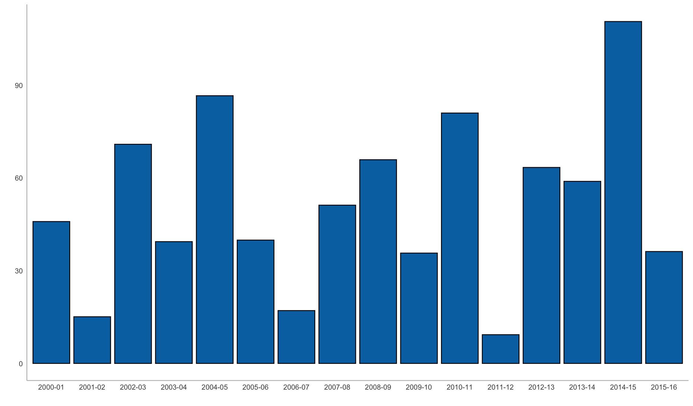Sharon Machlis

ggpackets is by Doug Kelkhoff and is accessible on CRAN.

Simpler ggplot2 code: ggblanket and others

ggplot2 is extremely highly effective and customizable, however generally that comes at a price of complexity. A number of packages goal to streamline ggplot2 so widespread information visualizations are both easier or extra intuitive.

When you are likely to overlook which geoms to make use of for what, I like to recommend giving ggblanket a attempt. Considered one of my favourite issues concerning the bundle is that it merges col and fill aesthetics right into a single col aesthetic, so I now not want to recollect whether or not to make use of a scale_fill_ or scale_colour_ perform.

One other ggblanket profit: Its geoms corresponding to gg_col() or gg_point() embrace customization choices inside the features themselves as an alternative of requiring separate layers. And which means I solely want to take a look at one assist file to see issues like pal is for outlining a shade palette and y_title units the y-axis title, as an alternative of looking assist information for a number of separate features. ggblanket could not make it simpler for me to keep in mind all these choices, however they’re simpler to discover.

Right here’s the best way to generate a histogram from the Palmer penguins information set with ggblanket, (instance taken from the bundle web site):

library(ggblanket)
library(palmerpenguins)
penguins |> 
  gg_histogram(x = body_mass_g, col = species)

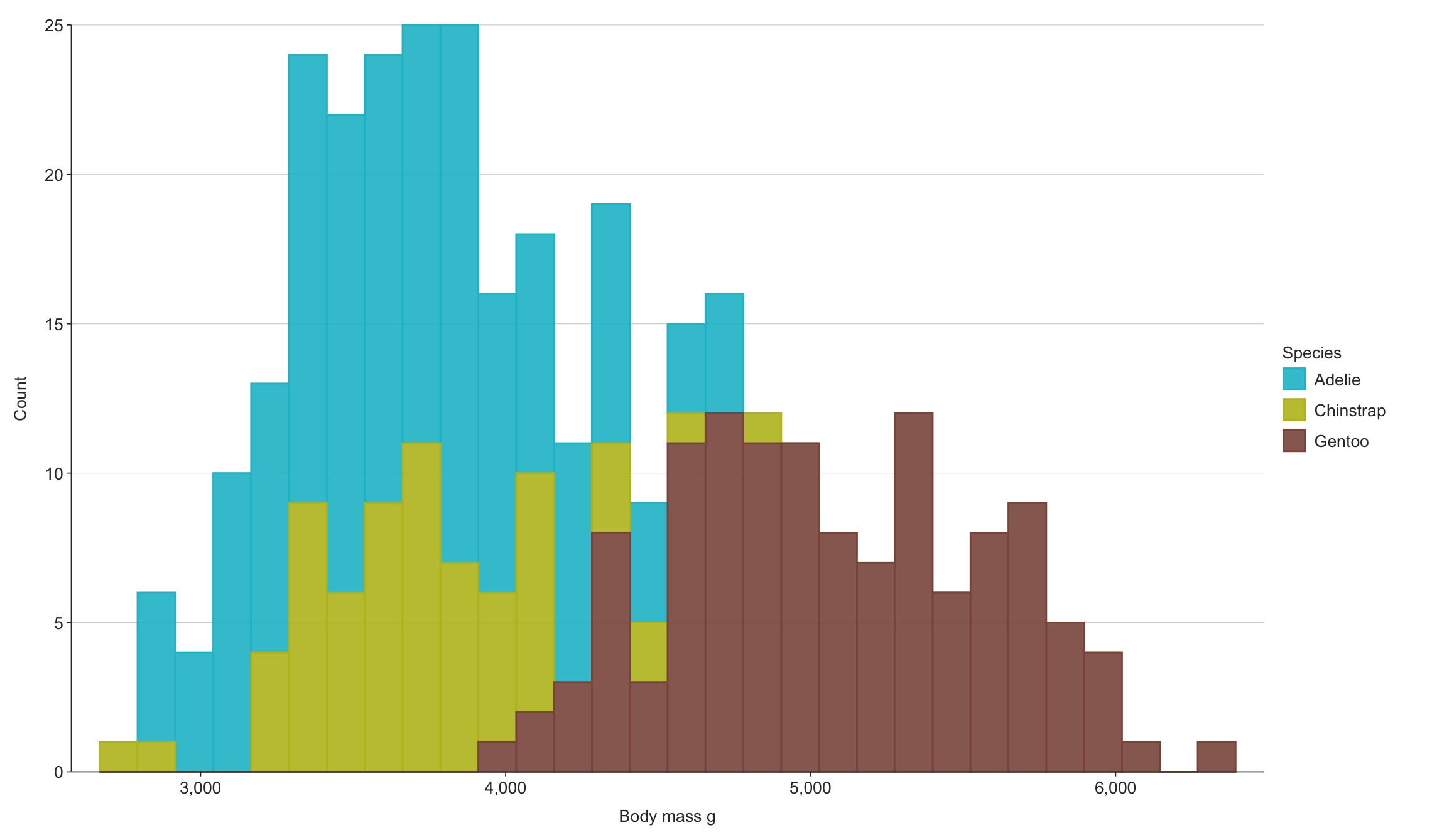Sharon Machlis

The end result remains to be a ggplot object, which suggests you’ll be able to proceed customizing it by including layers with standard ggplot2 code.

ggblankets is by David Hodge and is accessible on CRAN.

A number of different packages attempt to simplify ggplot2 and alter its defaults, too, together with ggcharts. Its simplified features use syntax like

library(ggcharts)
column_chart(snowfall2000s, x = Winter, y = Complete)

That single line of code supplies a reasonably respectable default, plus mechanically sorted bars (you’ll be able to simply override that).

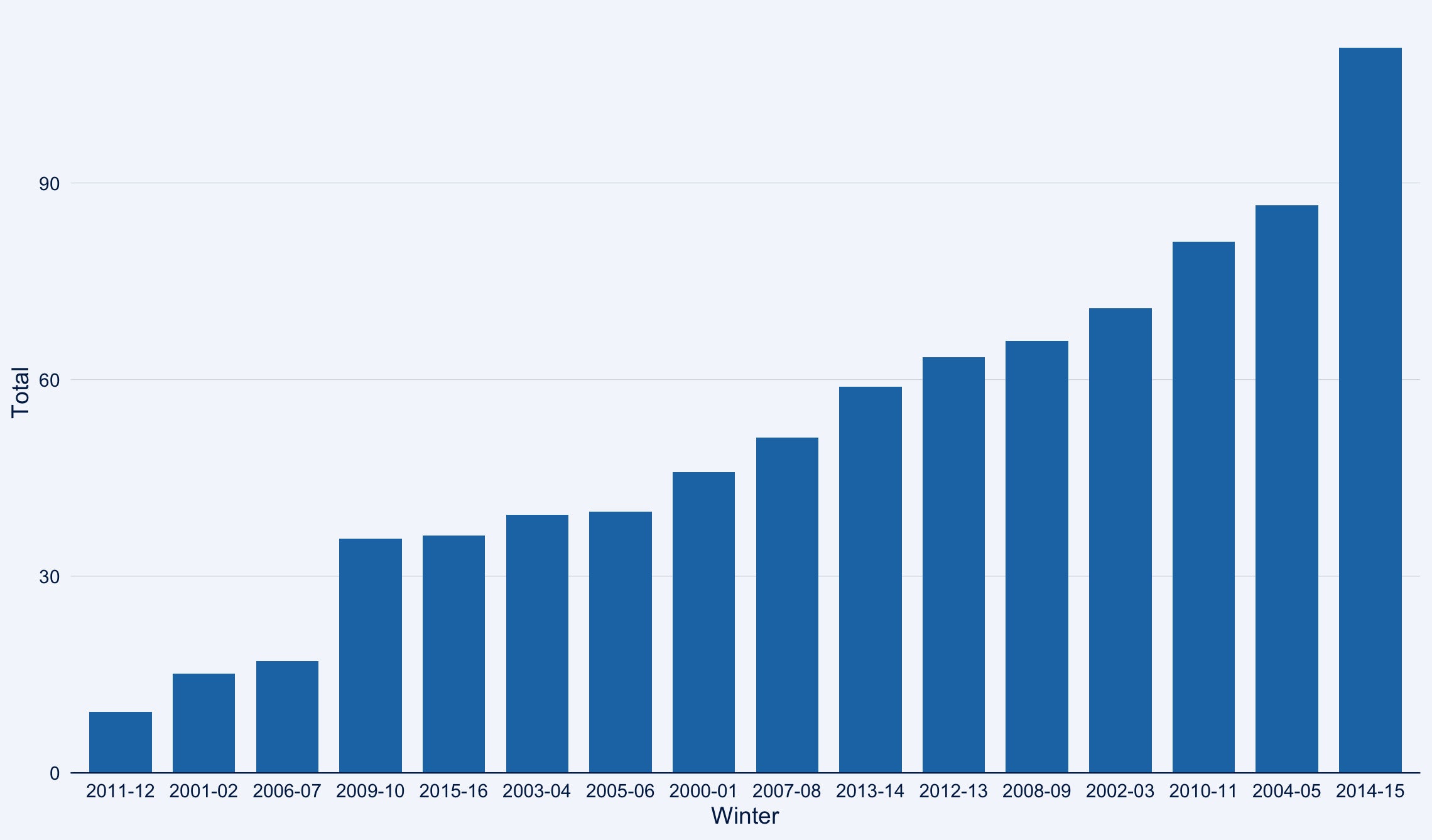Sharon Machlis

See the InfoWorld ggcharts tutorial or the video beneath for extra particulars.

Easy textual content customization: ggeasy

ggeasy doesn’t have an effect on the “important” a part of your dataviz—that’s, the bar/level/line sizes, colours, orders, and so forth. As a substitute, it’s all about customizing the textual content across the plots, corresponding to labels and axis formatting. All ggeasy features begin with easy_ so it’s, sure, simple to search out them utilizing RStudio auto-complete.

Have to heart a plot title? easy_center_title(). Wish to rotate x-axis labels 90 levels? easy_rotate_labels(which = "x").

Be taught extra concerning the bundle within the InfoWorld ggeasy tutorial or the video beneath.

ggeasy is by Jonathan Carroll and others and is accessible on CRAN.

Spotlight objects in your plots: gghighlight

Generally you wish to name consideration to particular information factors in a graph. You’ll be able to definitely try this with ggplot alone, however gghighlight goals to make it simpler. Simply add the gghighlight() perform together with a situation. For instance, if winters with complete snowfall greater than 85 inches are vital to the story I’m telling, I may use gghighlight(Complete > 85):

library(gghighlight)
ggplot(snowfall2000s, aes(x = Winter, y = Complete)) +
  my_geom_col() +
  gghighlight(Complete > 85)

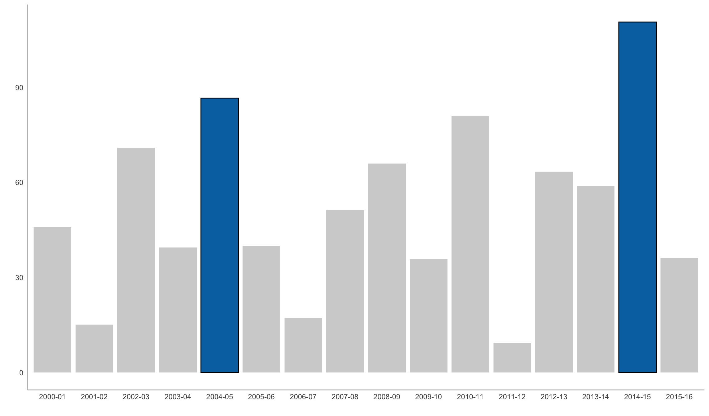Sharon Machlis

Or if I wish to name out particular years, corresponding to 2011-12 and 2014-15, I can set these as my gghighlight() situation:

ggplot(snowfall2000s, aes(x = Winter, y = Complete)) +
  my_geom_col() +
  gghighlight(Winter %in% c('2011-12', '2014-15'))

gghighlight is by Hiroaki Yutani and is accessible on CRAN.

Add themes or shade palettes: ggthemes and others

The ggplot2 ecosystem consists of a variety of packages so as to add themes and shade palettes. You seemingly gained’t want all of them, however you could wish to flick thru them to search out ones which have themes or palettes you discover compelling.

After putting in one in all these packages, you’ll be able to often use a brand new theme or shade palette in the identical method that you simply’d use a built-in ggplot2 theme or palette. Right here’s an instance with the ggthemes bundle’s solarized theme and colorblind palette:

library(ggthemes)
ggplot(penguins, aes(x = bill_length_mm, y = body_mass_g, shade = species)) +
  geom_point() +
  ggthemes::theme_solarized() +
  scale_color_colorblind()

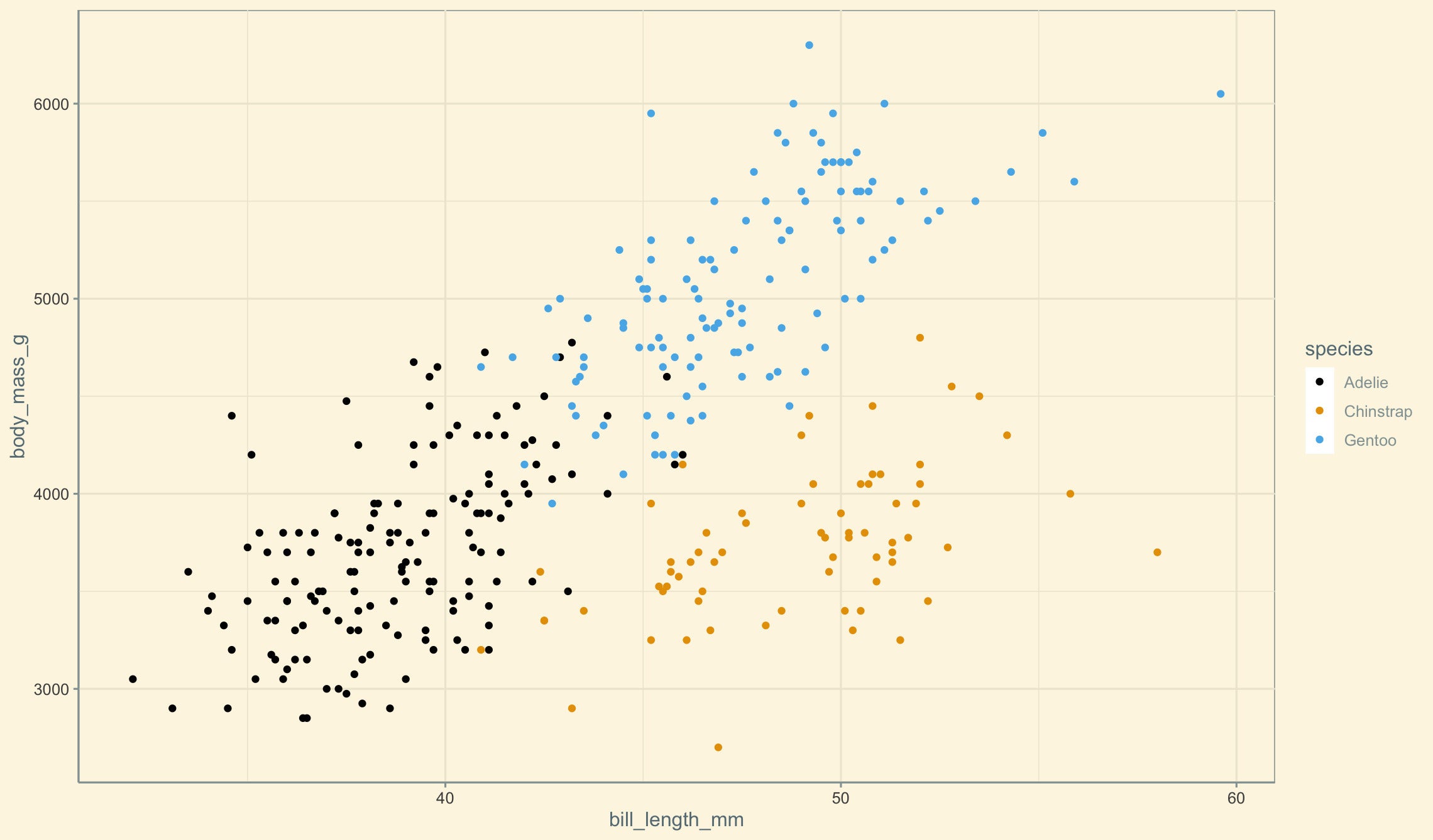Sharon Machlis

ggthemes is by Jeffrey B. Arnold and others and is accessible on CRAN.

Different theme and palette packages to think about:

ggsci is a set of ggplot2 shade palettes “impressed by scientific journals, information visualization libraries, science fiction motion pictures, and TV reveals” corresponding to scale_fill_lancet() and scale_color_startrek().

hrbrthemes is a well-liked theme bundle with a deal with typography.

ggthemr is a bit much less well-known than these others, however it has quite a lot of themes to select from plus a GitHub repo that makes it simple to browse themes and see what they appear like.

bbplot has only a single theme, bbc_style(), the publication-ready type of the BBC, in addition to a second perform to avoid wasting a plot for publication, finalise_plot().

paletteer is a meta bundle, combining palettes from dozens of separate R palette packages into one with a single constant interface. And that interface consists of features particularly for ggplot use, with a syntax corresponding to scale_color_paletteer_d("nord::aurora"). Right here nord is the unique palette bundle identify, aurora is the particular palette identify, and the _d signifies that this palette is for discreet values (not steady). paletteer is usually a little overwhelming at first, however you’ll nearly definitely discover a palette that appeals to you.

Observe that you should use any R shade palette with ggplot, even when it doesn’t have ggplot-specific shade scale features, with ggplot’s handbook scale features and the colour palette values, corresponding to scale_color_manual(values=c("#486030", "#c03018", "#f0a800")).

Add shade and different styling to ggplot2 textual content: ggtext

The ggtext bundle makes use of markdown-like syntax so as to add kinds and colours to textual content inside a plot. For instance, underscores surrounding the textual content add italics and two asterisks across the textual content create daring styling. For this to work correctly with ggtext, the bundle’s element_markdown() perform have to be added to a ggplot theme, too. Syntax is so as to add the suitable markdown styling to the textual content and then add element_markdown() to the ingredient of the theme, corresponding to this for italicizing a subtitle:

library(ggtext)
ggplot(snowfall2000s, aes(x = Winter, y = Complete)) +
  my_geom_col() +
  labs(title = "Annual Boston Snowfall", subtitle = "_2000 to 2016_") +
  theme(
    plot.subtitle = element_markdown()
  )

ggtext is by Claus O. Wilke and is accessible on CRAN.

Convey uncertainty: ggdist

ggdist provides geoms for visualizing information distribution and uncertainty, producing graphics like rain cloud plots and logit dotplots with new geoms like stat_slab() and stat_dotsinterval(). Right here’s one instance from the ggdist web site:

library(ggdist)
set.seed(12345) # for reproducibility
information.body(
  abc = c("a", "b", "b", "c"),
  worth = rnorm(200, c(1, 8, 8, 3), c(1, 1.5, 1.5, 1))
) %>%
  ggplot(aes(y = abc, x = worth, fill = abc)) +
  stat_slab(aes(thickness = stat(pdf*n)), scale = 0.7) +
  stat_dotsinterval(aspect = "backside", scale = 0.7, slab_size = NA) +
  scale_fill_brewer(palette = "Set2")

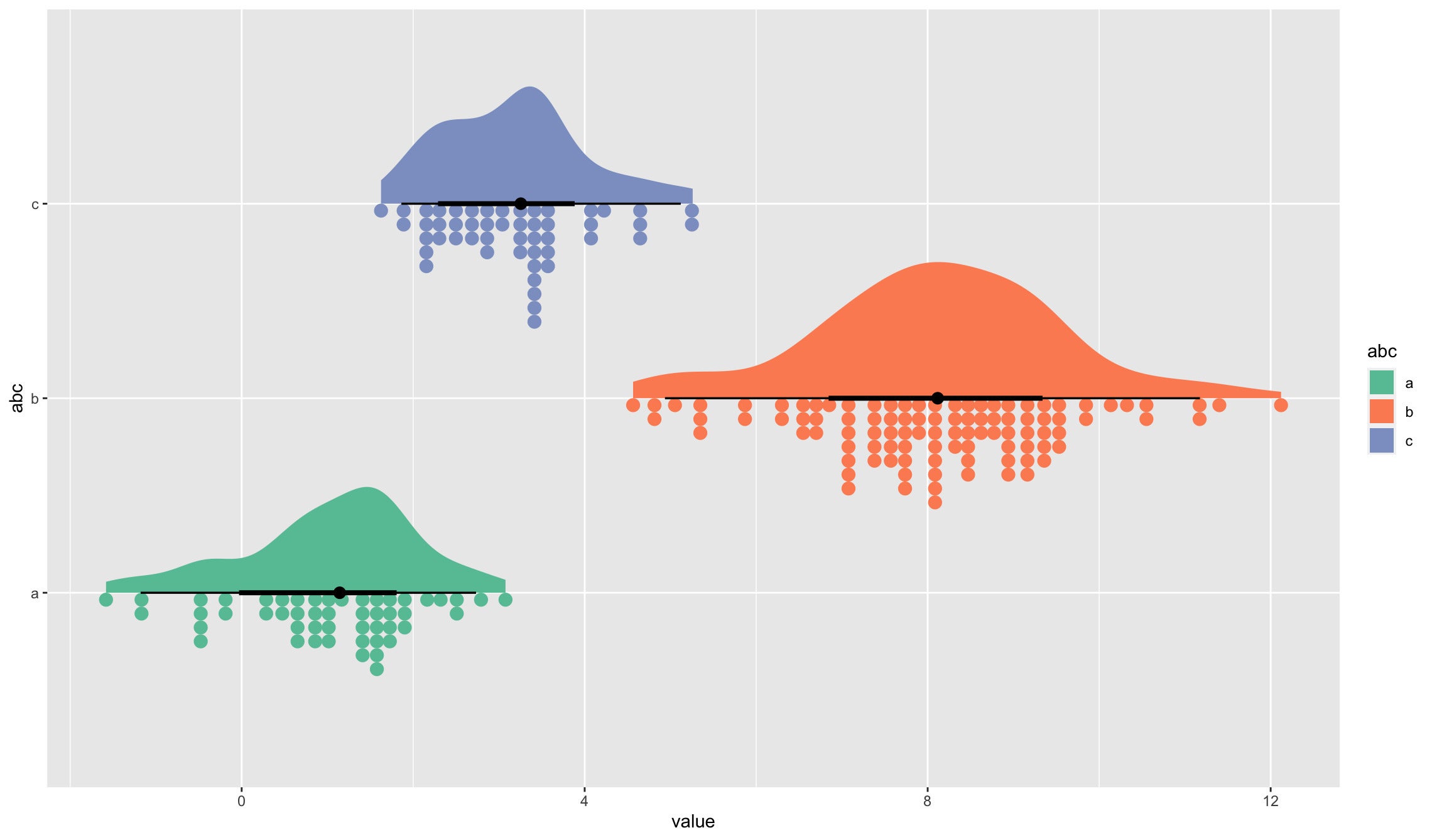Sharon Machlis

Try the ggdist web site for full particulars and extra examples. ggidst is by Matthew Kay and is accessible on CRAN.

Add interactivity to ggplot2: plotly and ggiraph

In case your plots are going on the internet, you may want them to be interactive, providing options like turning collection on and off and displaying underlying information when mousing over some extent, line, or bar. Each plotly and ggiraph flip ggplots into interactive HTML widgets.

plotly, an R wrapper to the plotly.js JavaScript library, is very simple to make use of. All you do is place your ultimate ggplot inside the bundle’s ggplotly() perform, and the perform returns an interactive model of your plot. For instance:

library(plotly)
ggplotly(
ggplot(snowfall2000s, aes(x = Winter, y = Complete)) +
  geom_col() +
  labs(title = "Annual Boston Snowfall", subtitle = "2000 to 2016")
)

plotly works with different extensions, together with ggpackets and gghighlights. plotly  graphs don’t all the time embrace every thing that seems in a static model (as of this writing it didn’t acknowledge ggplot2 subtitles, for instance). However the bundle is difficult to beat for fast interactivity.

Observe that the plotly library additionally has a non-ggplot-related perform, plot_ly(), which makes use of a syntax just like ggplot’s qplot():

plot_ly(snowfall2000s, x = ~Winter, y = ~Complete, sort = "bar")